A SAT Hardness Atlas: Runtime Landscapes and Ridge Structure Driven by Connectivity (V)

---

Full Text

A SAT Hardness Atlas: Runtime Landscapes and Ridge Structure Driven by Connectivity (V)

Christof Krieg Independent Researcher MAAT Research Initiative

II. Benchmark Setup

Abstract—We present an empirical hardness mapping pipeline for random SAT instances across a range of clause-to-variable ratios α. We introduce a Hardness Atlas that organizes SAT difficulty as a landscape over (α, V ), where V captures structural connectivity of constraints. Across 2000 benchmarked instances we observe: (i) a phase transition in satisfiability probability as α increases, (ii) a ridge-like structure of maximal median runtime in the hardness landscape, and (iii) predictive signal for runtime from field-based features. Our results indicate that connectivity V is a primary organizing variable for hardness in the sampled regime, while the derived complexity projection ˆC serves as a secondary explanatory axis. Index Terms—SAT, phase transition, hardness land- scape, runtime prediction, connectivity, empirical bench- marking

A. SAT Instance Type

All experiments are performed on random 3-SAT in- stances with n = 30 variables. Each clause contains exactly three literals chosen uniformly from the variable set. The number of clauses is determined by

m = αn

where α is the clause-to-variable ratio.

B. Instance Generation and Solving

We sample 2000 instances across a range of α values covering the phase transition region. Instances are solved using the MiniSAT 2.2 solver with default parameters. Runtime is measured as wall-clock solving time.

Boolean satisfiability (SAT) was the first problem shown to be NP-complete [1]. Subsequent work established a broad class of NP-complete problems [2]. Random SAT instances exhibit a phase transition in satisfiability probability as the clause-to-variable ratio varies [3], [4].Hard instances tend to concentrate near the phase transition region [5]. This paper contributes a compact empirical framework to:

C. Field Features

For each SAT instance we compute a set of scalar structural features interpreted as fields:

(H, B, S, V, R)

• construct a Hardness Atlas over (α, V ), treating V as a primary structural field,

D. Feature Definitions

• detect a hardness ridge (maximal median runtime locus) within the atlas,

The fields are derived from structural properties of the clause-variable interaction graph. Harmony (H) measures clause polarity balance across variables. Balance (B) captures the variance of clause sizes, reflecting constraint heterogeneity. Structure (S) measures clause overlap between clauses sharing variables. Connectivity (V) measures structural coupling be- tween variables. We construct a variable interaction graph where two variables are connected if they appear in the same clause. Connectivity is defined as

• evaluate runtime predictors using field features and compare to the secondary projection ˆC.

I. Related Work

Phase transitions in random SAT were first systemati- cally studied by Cheeseman et al. [3] and Gent and Walsh [4]. Subsequent work showed that the hardest instances tend to concentrate near this transition region [5]. Feature-based runtime prediction has been explored in SAT solver portfolio systems such as SATzilla [6]. These approaches rely on structural instance features to estimate solver difficulty. Our work differs by constructing an explicit hardness landscape over (α, V ) and identifying ridge structures in this space.

V = avg degree of interaction graph

n −1

where n is the number of variables. Respect (R) measures literal distribution uniformity across clauses.

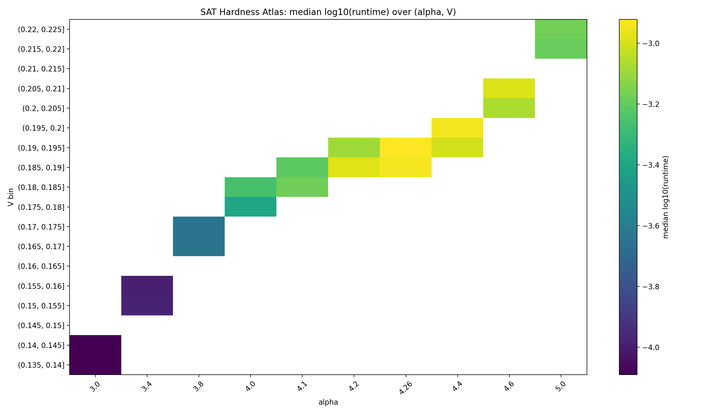
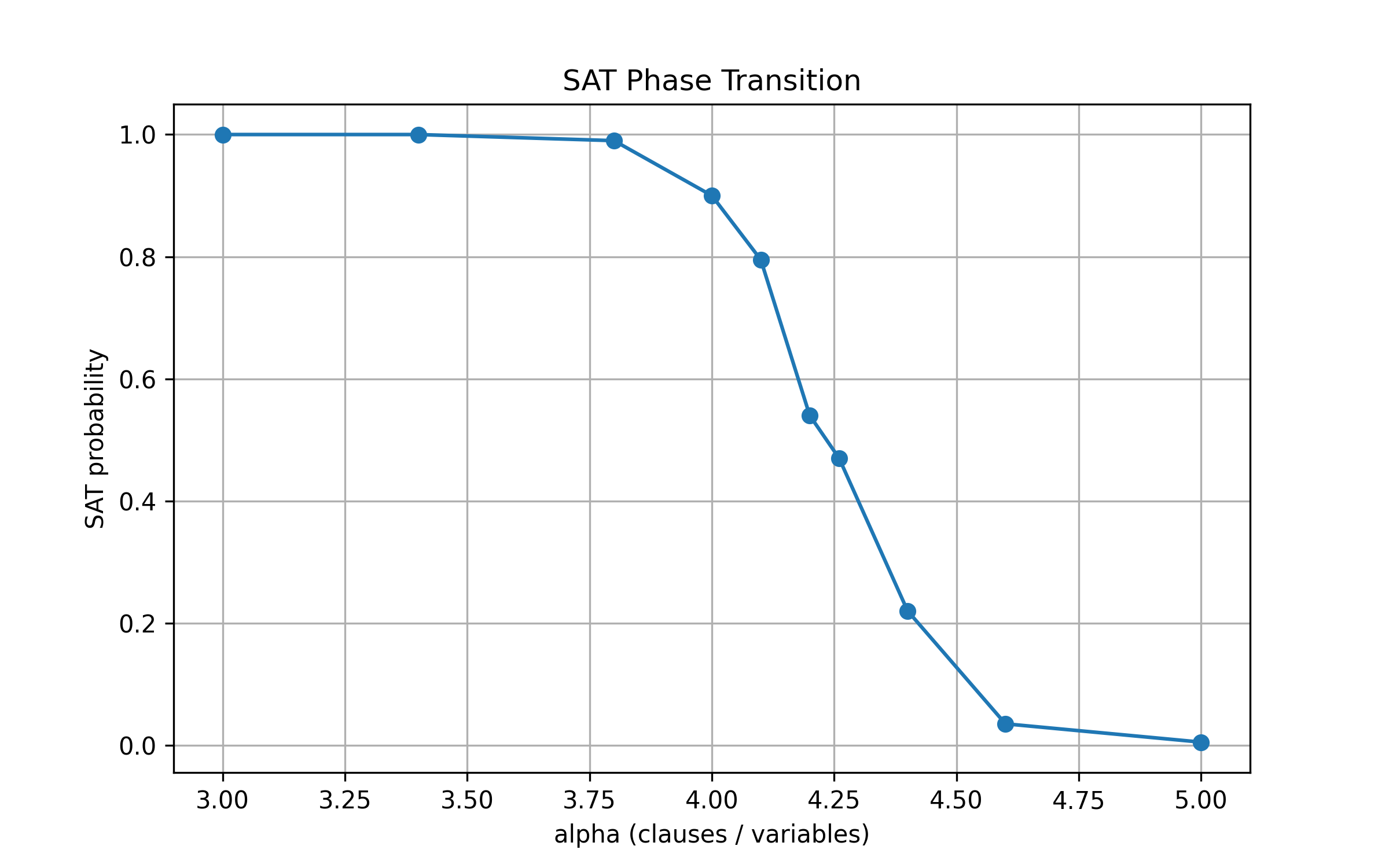
Fig. 2. Hardness Atlas: median log10(runtime) over (α, V ).

Fig. 1. SAT phase transition: P(SAT) vs. α.

E. Derived Complexity Projection

In addition to the structural fields we compute a scalar complexity projection

ˆC = H + B + S + V + R

5

which provides a compact summary of structural features. This projection is used only for visualization and secondary ridge analysis.

F. Aggregation

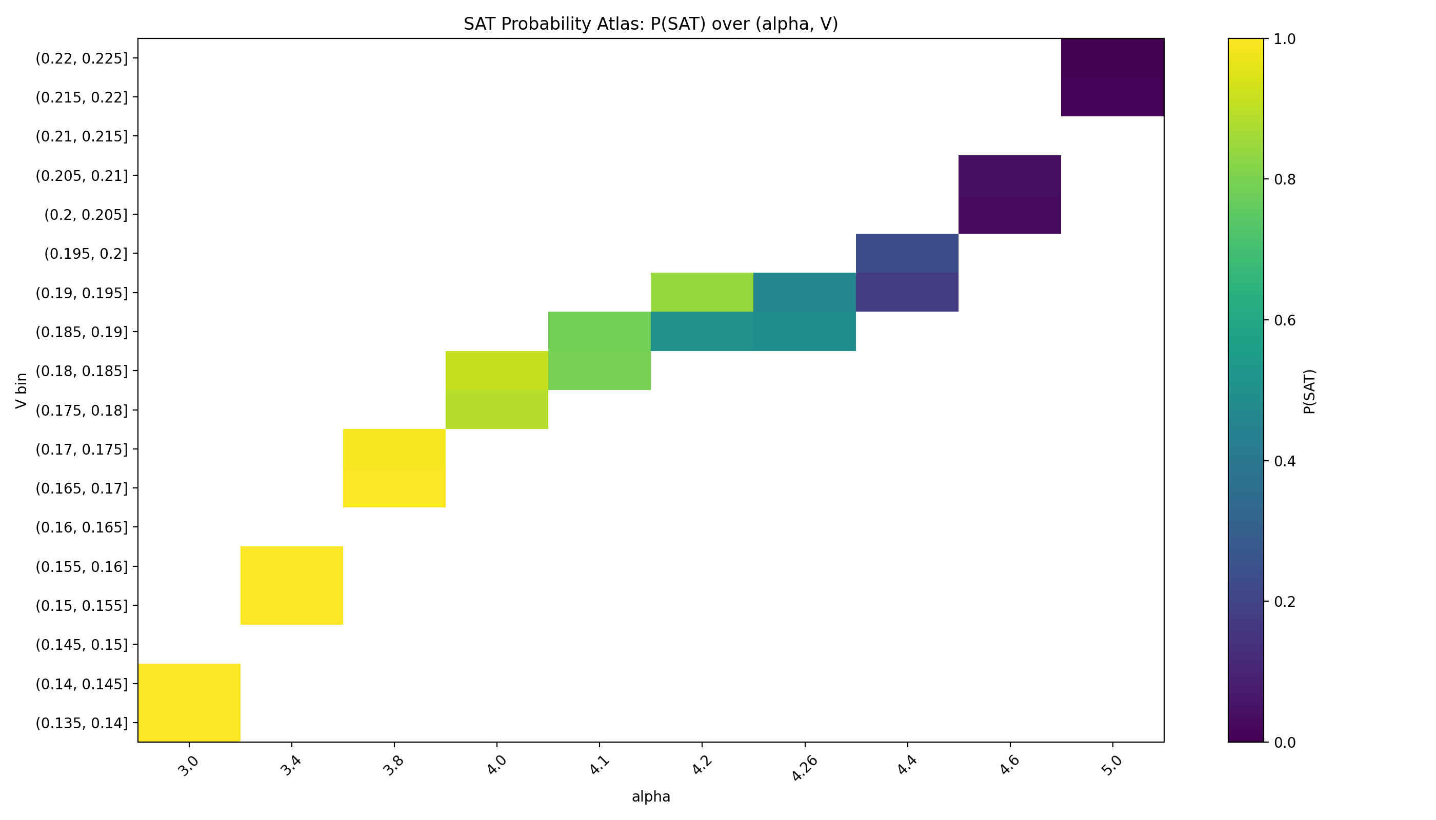
Fig. 3. SAT Probability Atlas: P(SAT) over (α, V ).

We aggregate results by binning:

• α into discrete bins (the swept values),

D. Secondary Projection: ˆC

• V into quantile or fixed-width bins,

• (optionally) ˆC into bins for a secondary landscape projection. Per bin we compute median runtime (log-scale) and SAT probability P(SAT).

As a secondary view, we project the landscape onto (α, ˆC). This supports interpretability and connects field- based structure to a compact scalar.

E. Predicting Runtime from Fields

III. Results

We fit a linear model on log-runtime using field features and α:

A. SAT Phase Transition

log10(runtime) ≈β0+βαα+βHH+βBB+βSS+βV V +βRR.

Figure 1 shows the satisfiability probability versus α, exhibiting a sharp transition region as α increases.

In the current benchmark, the fitted OLS model achieves R2 ≈ 0.583. We also evaluate a regularized regres- sion model (ridge regression) using the same feature set (α, H, B, S, V, R). Regularization reduces multicollinearity effects and improves predictive performance to R2 ≈0.655.

B. Hardness Atlas over (α, V )

We define the Hardness Atlas as a grid over (α, V ), with cell values given by median log10(runtime) and (separately) P(SAT). Figure 2 plots the median runtime atlas; Figure 3 shows P(SAT) on the same grid; Figure 4 shows per-cell sample counts.

F. 3D Phase Surface

For visualization, we render a phase surface over (α, V ) where height is median log-runtime. Figure 7 provides an intuitive 3D view of the ridge structure.

C. Hardness Ridge Detection

IV. Empirical Hardness Field Equation

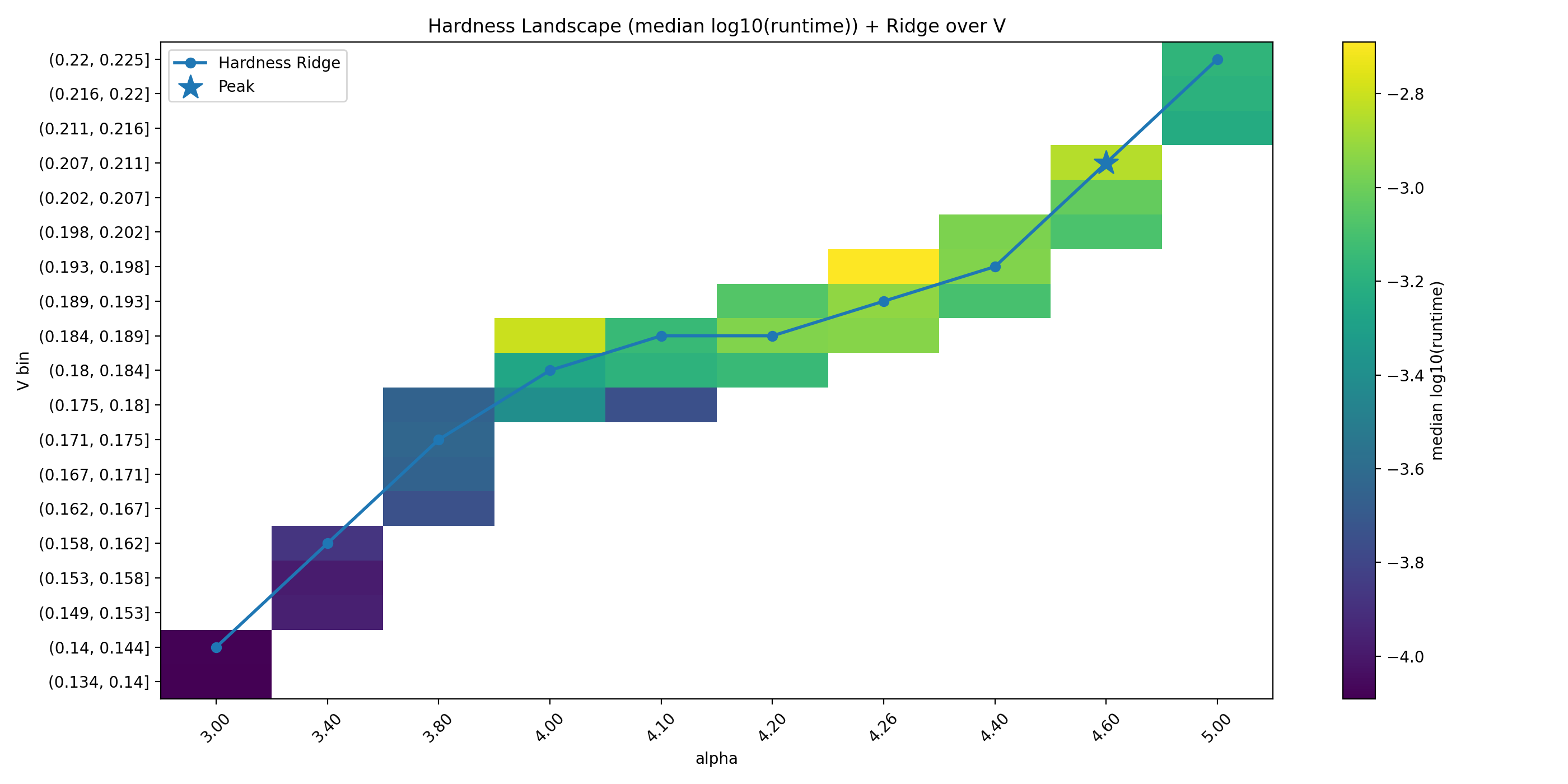
We define the hardness ridge as the locus of maximal median runtime along the V dimension for each fixed α bin. Figure 5 overlays the ridge on the atlas and marks the peak cell.

The hardness atlas suggests that SAT difficulty in the sampled regime can be described by a low-dimensional structural relation.

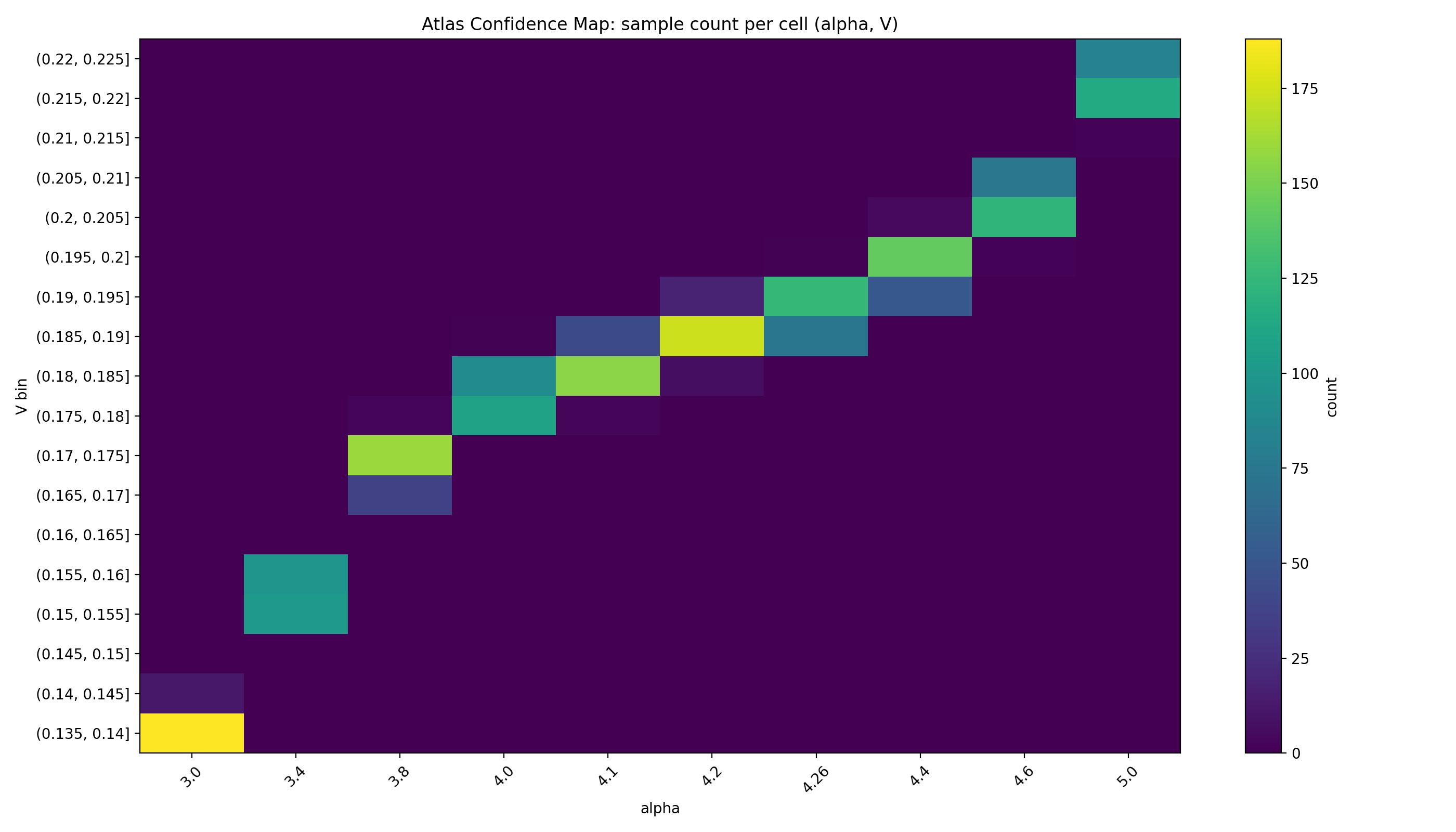
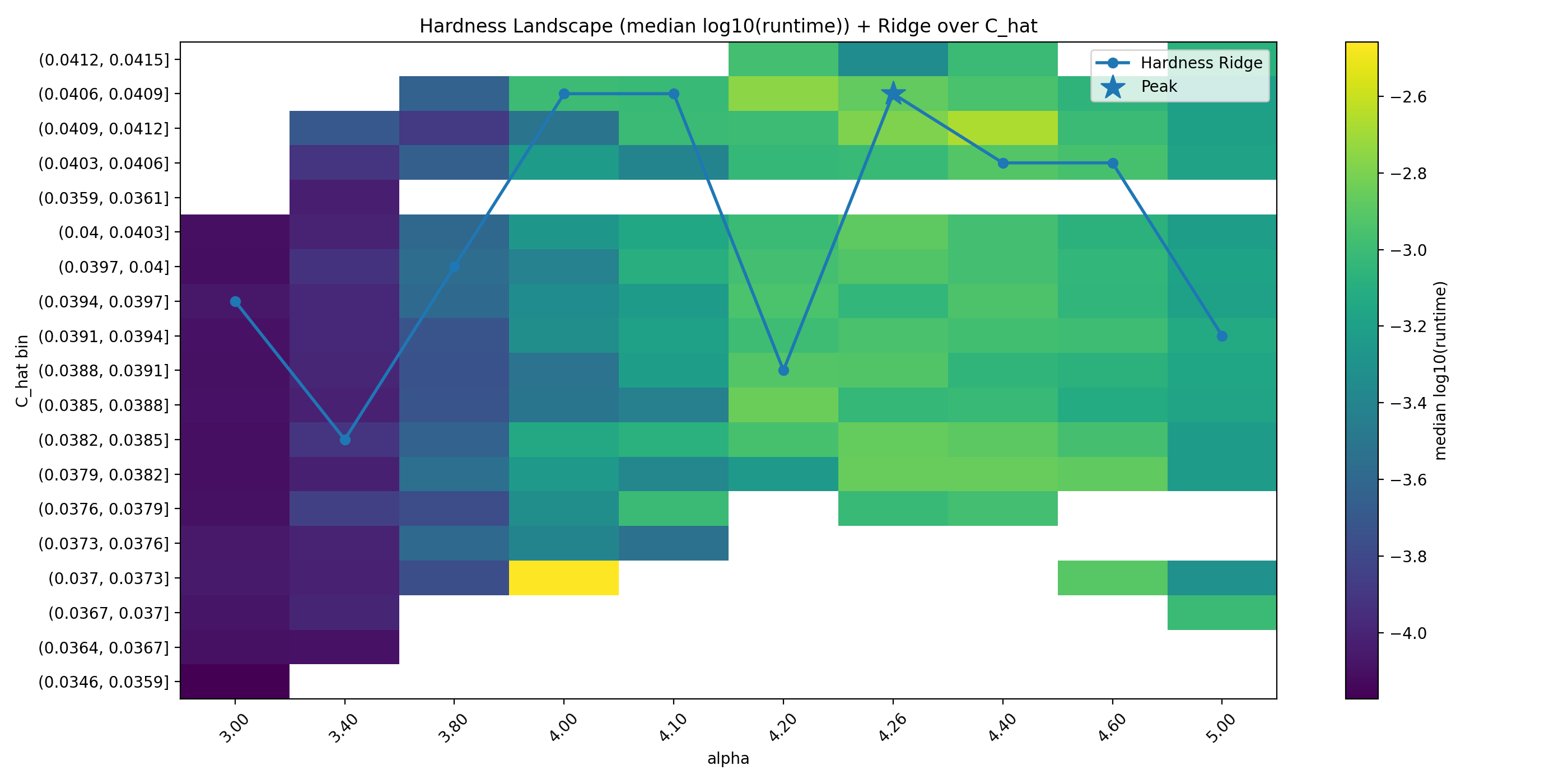
Fig. 6. Secondary ridge over ˆC (projection view).

Fig. 4. Atlas confidence map: sample count per (α, V ) cell.

TABLE I OLS regression coefficients for log-runtime prediction.

Feature Coefficient Std. Error

Intercept -4.179 13.484 α -1.689 0.175 H -20.383 1.125 B 0.396 0.417 S 12.315 13.494 V 13.937 4.141 R 0.790 0.612

statistically significant in the present sample. This supports the interpretation that connectivity V is the most robust structural signal for hardness in our experiments. The large standard error of the intercept suggests multicollinearity among the structural features. This is expected because several fields are derived from related structural properties of the clause-variable interaction graph. This observation motivated the use of ridge regres- sion as a regularized alternative, which stabilizes coefficient estimates in the presence of correlated predictors.

Fig. 5. Hardness ridge over V : per-α maximal median runtime locus and peak marker.

Empirically we observe that runtime depends primarily on clause density α and structural connectivity V :

log10(runtime) ≈β0 + βαα + βV V + ϵ(H, B, S, R)

where ϵ represents secondary corrections from additional structural fields. In this view the hardness ridge corresponds to a locus of maximal runtime in (α, V ) space, which we detect empirically using the ridge extraction procedure described above.

VI. Limitations

Our results are empirical and therefore depend on the instance generator, solver choice, feature definitions, and sampling density used in the benchmark. Sparse cells in the atlas require cautious interpretation; confidence maps should accompany atlas plots. The current benchmark uses 2000 instances as an ex- ploratory dataset. Scaling the hardness atlas to significantly larger instance ensembles is an important direction for future work. The small instance size (n = 30 variables) limits the generalizability of the observed hardness landscape. While phase transition behavior is visible even at this scale, larger instances may exhibit qualitatively different ridge structures or sharper phase boundaries. Future work should extend the hardness atlas to larger instance sizes to evaluate the stability of the (α, V ) ridge phenomenon. Nevertheless, the atlas framework itself is independent of instance size and can be applied to larger SAT ensembles in future studies.

V. Discussion

The results provide an empirical view of the structural organization of SAT hardness in the sampled regime. The atlas results suggest that hardness is organized jointly by clause density α and structural connectivity V . Near the phase transition region, increasing connectivity strengthens global constraint coupling, which may lead to stronger constraint propagation effects during solving. This interaction naturally produces a ridge-like band of maximal runtime in (α, V ) space. The regression coefficients indicate that H and V have statistically significant contributions in the current dataset. In contrast, S exhibits a large standard error relative to its coefficient, suggesting that its contribution is not

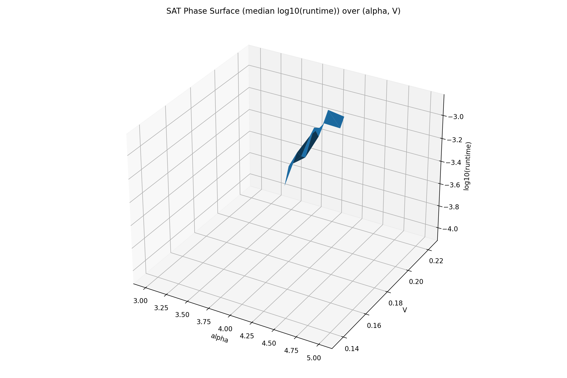
Fig. 7. Phase surface: median log10(runtime) over (α, V ).

VII. Conclusion

We introduced a SAT Hardness Atlas centered on (α, V ) and demonstrated ridge structure in median runtime landscapes. Predictive experiments indicate that V is a dominant signal for runtime in the current benchmark, with ˆC serving as a helpful secondary projection. All code and full-resolution figures are provided in the companion repository.

Artifacts and Reproducibility

All datasets, code, and analysis scripts used in this study are publicly available at:

https://github.com/Chris4081/sat-hardness-atlas The repository includes:

• SAT instance generation scripts

• benchmark and solver pipeline

• hardness atlas analysis code

• plotting scripts used to generate the figures

• CSV datasets containing all benchmark results These artifacts allow the complete experimental pipeline to be reproduced.

References

[1] S. A. Cook, “The complexity of theorem-proving procedures,” Proceedings of the Third Annual ACM Symposium on Theory of Computing, 1971. [2] R. M. Karp, “Reducibility among combinatorial problems,” 1972. [3] P. Cheeseman, B. Kanefsky, and W. M. Taylor, “Where the really hard problems are,” IJCAI, 1991. [4] I. P. Gent and T. Walsh, “Phase transitions and the search problem,” Artificial Intelligence, 1996. [5] D. Mitchell, B. Selman, and H. Levesque, “Hard and easy distributions of SAT problems,” AAAI, 1992. [6] L. Xu, F. Hutter, H. Hoos, and K. Leyton-Brown, “Satzilla: Portfolio-based algorithm selection for sat,” Journal of Artificial Intelligence Research, vol. 32, pp. 565–606, 2008.