Every day, hundreds of millions of posts compete for a finite resource: human attention. We present a descriptive analysis of how this resource is distributed among English-language posts on X (formerly Twitter), drawing on a cross-sectional sample of 8,722 tweets (February 2026, after bot filtering), a timeline panel of 17,671 tweets from 225 users, and a historical archive of 95 million tweets (2009–2018). Four main findings and one cautionary observation emerge: (1) attention inequality is extreme among text-containing posts—the impression Gini is 0.965, and after inverse-probability weighting (IPW) to correct for the stratified over-sampling of high-follower accounts, approximately 81% of total variance is between users rather than between posts (unweighted upper bound: 88%, bootstrap 95% CI: [84%, 89%]); (2) the association between followers and impressions shows increasing returns in the 100–100,000 follower range, with possible saturation above 100K— a cross-section analysis (n = 7,673) yields ˆ β2 = 0.053 (p < 0.001, R2 = 0.761) for a global quadratic approximation; this pattern persists under all filter specifications, including automation-only filtering ( ˆ β2 = 0.030, p < 0.001); (3) retweet inequality rose within the EPFL archive (verified-account Gini: 0.76 in 2012, 0.89 in 2018), a pattern consistent with both platform evolution and cohort maturation; (4) likes, quotes, and impressions are tightly coupled in equilibrium, with the coupling weakening for larger accounts—attributable to mechanical necessity (one must see a tweet to like it) and selection effects, with algorithmic amplification as one possible additional channel. We also note that follower inequality decreased within the fixed EPFL cohort, though this is likely a survivorship artifact. Pooling with the stratified timeline panel raises R2 to 0.821. These findings describe a platform where attention is concentrated far beyond what follower counts alone would predict—consistent with algorithmic mediation, though our evidence is descriptive rather than causal.
1 Introduction
In 1971, Herbert Simon observed that "a wealth of information creates a poverty of attention" (Simon, 1971). Half a century later, his insight has become the organizing principle of the digital economy. Social media platforms are, at their core, attention allocation machines: they decide which of millions of competing posts will appear on a user's screen and which will vanish unseen. The distributional consequences of these decisions—who is heard, who is ignored, and how concentrated the resulting attention distribution becomes—are questions of both scientific and democratic significance.
Yet for all the debate about algorithmic power, the basic distributional facts remain surprisingly understudied. Follower counts are known to follow heavy-tailed distributions (Kwak et al., 2010; Barabási and Albert, 1999), and online participation is extraordinarily concentrated—the "90-9-1 rule" describes a world where 1% of users create most content (Nielsen, 2006). But the distribution of realized attention—not who could be heard, but who actually is—has received far less scrutiny. This gap exists largely because impression data (how many times a post is rendered on a screen) was proprietary until X began exposing it through its API in late 2022.
We exploit this opening to offer a descriptive anatomy of attention inequality on X/Twitter, organized around five stylized facts. We combine a cross-sectional sample of 8,722 tweets with impression counts (after bot filtering), a panel of 17,671 tweets from 225 user timelines to decompose inequality into its between-user and within-user components, and a historical archive of 95 million tweets spanning a decade of platform evolution.
A clarification on what we measure: impressions count screen renders, not cognitive engagement. A tweet that flashes past in a feed and one that holds a reader's attention for minutes both register as a single impression.[^1] Nevertheless, impressions are the currency that determines a creator's visibility and mediates a reader's exposure to ideas and political speech—making them the relevant quantity for questions about platform power.
Zhu and Lerman (2016) provided an important benchmark, reporting a user-level retweet Gini of ∼0.94 on 2014 data and documenting rich-get-richer dynamics. We extend their work in three directions: measuring inequality with impression data, tracing temporal trends from 2009 to 2026, and characterizing the equilibrium coupling between engagement signals and exposure. Among our findings, the degree of concentration stands out: the impression Gini (0.965) exceeds Gini values reported for other digital attention distributions such as YouTube views (∼0.87; Cha et al. 2010) and scientific citations (∼0.70–0.80; de Solla Price 1976). For context, this also exceeds the income Gini of any country on record, though the comparison is imperfect: attention distributions are structurally more zero-inflated than income distributions, which inflates the Gini mechanically (see Section 4). Furthermore, approximately 81% of the variance in impressions is between users rather than between posts after IPW-weighting (unweighted upper bound: 88%; Section 4), and even a model with rich controls can explain only 82% of the variation—the remaining 18% reflecting the inherent unpredictability of individual posts.
2 Related Work
The economics of attention traces back to Simon (1971) and was developed for digital environments by Goldhaber (1997) and Davenport and Beck (2001). The empirical regularity that online participation follows extreme power laws is one of the most robust findings in computational social science: from the "90-9-1 rule" (Nielsen, 2006) to the participation divide (Hargittai and Walejko, 2008) to Hindman's (2009) demonstration that online discourse is more concentrated than its offline counterpart.
These distributional patterns have deep structural roots in cumulative advantage processes. Simon (1955) first modeled cumulative advantage mathematically, showing that a process where the probability of acquiring new items is proportional to how many one already has generates skew distributions. Merton (1968) identified the same dynamic in the sociology of science as the "Matthew Effect." de Solla Price (1976) showed that scientific citations follow this cumulative advantage process, with highly cited papers attracting citations at a disproportionate rate. Barabási and Albert (1999) generalized the mechanism to networks as "preferential attachment," demonstrating that growing networks where new nodes connect preferentially to well-connected nodes produce power-law degree distributions. In cultural markets, Salganik et al. (2006) demonstrated experimentally that social influence can amplify small initial differences into extreme inequality, while Muchnik et al. (2013) showed that even a single artificial upvote can bias the trajectory of a post's success. The economic formalization appears in Rosen (1981): when audiences can costlessly concentrate on top performers, small quality differences generate extreme outcome inequality—the "superstar" effect.
The transition from chronological to algorithmic feeds introduces a new form of endogenous reinforcement. When platforms use engagement signals to rank content, a feedback loop emerges: early engagement increases visibility, which generates further engagement, which further increases visibility. These dynamics can endogenously produce cumulative advantage and heavy-tailed attention distributions even absent intrinsic quality differences between posts. Empirical evidence supports this mechanism: Huszár et al. (2022) documented asymmetric political amplification in Twitter's algorithm; Garz and Dujeancourt (2023) exploited the 2016 algorithmic switch as a natural experiment, finding both increased engagement and a rich-get-richer pattern; and more broadly, the transition from social-graph-based feeds to interest-graph-based recommendation—what Gerbaudo (2024) calls the shift from "social networks" to "social interest clusters"—has fundamentally restructured how platforms allocate visibility, decoupling who sees a post from who follows its author.
A deeper literature on recommender systems illuminates the mechanism. Chaney et al. (2018) showed formally that recommendation algorithms create "algorithmic confounding": by mediating what users see, they generate observational data that reinforces existing popularity even absent intrinsic quality differences. Fleder and Hosanagar (2009) found that collaborative filtering can increase sales concentration despite expanding the range of items recommended. These feedback loops mean that ranking algorithms using engagement signals as inputs can endogenously produce rich-get-richer dynamics—not as a design choice, but as an emergent property. The diffusion structure of content matters too: Goel et al. (2016) showed that most viral events are shallow and broad rather than deeply cascading, suggesting that algorithmic distribution, not organic word-of-mouth, drives the bulk of attention concentration.
3 Data and Methods
3.1 Data Sources
We draw on four datasets, summarized in Table 1.
Cross-sectional sample. This dataset consists of 11,007 English-language original tweets collected via the X API v2 across 110 randomly selected one-minute windows spanning February 22–28, 2026 (8,722 tweets from 8,547 authors after data cleaning; see below). For each window, we queried the tweets/search/recent endpoint using a disjunction of ten common English stopwords—(the OR just OR that OR this OR was OR with OR but OR what OR been OR they) lang:en -is:retweet -is:reply—filtered to exclude retweets and replies. This stopword-matching strategy approximates a random sample of the English-language tweet stream: because the target words appear in a large fraction of English sentences, the query acts as a near-uniform filter over the population of English text-containing tweets posted in each window. This approach inherently excludes non-English content and may underrepresent media-only posts (images/videos without text) or posts using non-standard syntax; if such posts tend to have higher engagement, our inequality estimates would be conservative. The resulting sample contains approximately one tweet per author, making tweet-level and user-level distributions effectively equivalent. Because the X API only returns tweets from accounts that exist at the time of collection, our sample does not include posts from accounts that were active during the collection week but subsequently deleted or suspended (survivorship bias); results therefore describe accounts that maintained an active presence and should not be extrapolated to accounts that churned.
For each tweet, the API returns cumulative engagement metrics (impressions, likes, retweets, replies, quotes, bookmarks) and author metadata (followers, following, total tweets, account age). Impressions are measured at a single observation point (collection time); tweet ages range from 3.5 to 143 hours (mean 74h). The 110 windows were distributed across all hours and days of the week; a Theil decomposition by time of day explains only 1.8% of total inequality (Table 6), confirming that temporal clustering does not drive our results. We assess sensitivity to tweet age in Table 3.
User timeline panel. To separate post-level from user-level inequality, we collected a panel of 19,343 tweets from 243 authors sampled stratified by follower count (17,671 tweets from 225 users after cleaning). From each of six log-spaced strata, we drew up to 32 users and retrieved up to 100 recent original tweets per author via users/:id/tweets. Of the 270 users initially sampled, 27 returned zero tweets and were excluded. Tweets were restricted to those at least one week old to ensure near-complete engagement accumulation.[^2] Because the stratified design over-represents high-follower accounts relative to the population, the variance decomposition estimates are conditional on this sample composition and should be interpreted as characterizing the structure of inequality (between-user vs. within-user) rather than as population-weighted statistics. To provide a population-corrected estimate, we apply inverse-probability weights (IPW) based on the ratio of cross-section strata proportions (a proxy for the population distribution) to panel strata proportions; this yields an IPW-weighted between-user variance share of 81%, reported in Section 4.
EPFL historical archive. For temporal analysis, we use the publicly available "Evolution of Retweet Rates" dataset (Garimella and West, 2021), containing 95 million tweets (2009–2018) with retweet counts and estimated follower counts at time of posting. Data spans three author cohorts: a random sample (18.8M tweets, 9,345 users; used in full), verified accounts (7.0M tweets, 3,597 users; used in full), and political accounts (69.2M tweets, 30,320 users; used as a systematic 1-in-5 subsample due to computational constraints). Engagement counts in stream-captured data are frozen near zero at capture time; we therefore compute both unconditional metrics and metrics conditional on RT ≥ 1. Three corrupt rows in the random cohort (where tweet IDs were parsed as retweet counts exceeding 5 million) were removed.
Economist validation sample. To provide a "guaranteed human" benchmark, we collected timelines for 144 of the top 150 economists ranked by Twitter followers in the RePEc/IDEAS ranking (IDEAS/RePEc, 2022), obtaining 12,438 tweets.[^3] These accounts are verified public intellectuals, reducing concerns about bots or purchased followers. The economist sample is used exclusively as a visual validation overlay on Figure 3; it is not included in the regression models or inequality statistics, because it is a purposive sample of high-profile users that would distort the random-sample representativeness of the cross-sectional and stratified timeline datasets.
Data cleaning. We applied an aggressive composite filter to remove likely bots, purchased-follower accounts, and suspended users from the cross-sectional and timeline data. An account was flagged if any of the following held: (i) mean impressions-to-followers ratio below 0.5% with >100 followers (purchased/dead audience); (ii) 100% zero likes across all observed tweets with >500 followers (ghost accounts); (iii) lifetime posting rate above 200 tweets per day (automated posting); or (iv) all observed tweets with <10 impressions despite >1,000 followers (shadowbanned/suspended). This removed 2,207 authors (20.5% of unique accounts) and 3,955 tweets (13.0%), but only 1.3% of total impressions—consistent with these accounts contributing negligible real attention. We acknowledge a circularity risk in criterion (i): removing accounts with low impression-to-follower ratios when studying the follower–impression relationship could censor the lower bound of the performance distribution. However, the filter removes accounts whose audience is overwhelmingly inactive (0.5% reach among >100 followers), and the sensitivity analysis (Table 4) shows inequality is higher without any filtering (Gini 0.967 vs. 0.965), confirming the filter does not inflate concentration. The filter's effect is better understood as removing "invisible" accounts from a study of "visibility"—our results describe inequality among accounts that reach a human audience, not among all registered accounts. For the regression results, we additionally report estimates omitting criterion (i) entirely (Table 5, notes; see also Appendix B): the convex association (\(\hat{\beta}_2 = 0.028\), p < 0.001) persists, though it is attenuated relative to the full-filter sample, as expected if criterion (i) removes some genuinely low-reach accounts. After cleaning, the cross-sectional sample contains 8,722 tweets from 8,547 authors and the timeline panel contains 17,671 tweets from 225 users. All results below use the cleaned samples unless otherwise noted.
Table 1: Summary of data sources (post-cleaning counts in parentheses)
| Dataset | Period | Tweets | Authors | Key metric |
|---|---|---|---|---|
| Cross-section | Feb 2026 | 8,722 | 8,547 | Impressions |
| Timeline panel | Feb 2026 | 17,671 | 225 | Impressions |
| Economist valid.‡ | Feb 2026 | 12,438 | 144 | Impressions |
| EPFL random | 2009–18 | 18.8M | 9,345 | Retweets |
| EPFL verified | 2009–18 | 7.0M | 3,597 | Retweets |
| EPFL political | 2009–18 | 13.8M† | 30,320 | Retweets |
†Systematic 1-in-5 subsample of 69.2M tweets. ‡Top 150 RePEc economists by Twitter following (IDEAS/RePEc, 2022); used only for visual validation (Figure 3), not in regressions or inequality statistics. Pre-cleaning cross-section: 11,007 tweets, 10,754 authors; timeline panel: 19,343 tweets, 243 users.
3.2 Inequality Measures
We deploy a battery of inequality measures, each illuminating a different facet of the distribution. The Gini coefficient (G) captures overall concentration; the Palma ratio (top 10% share divided by bottom 40% share) highlights the distance between the most visible accounts and the majority that receives little attention; top-k% shares describe the upper tail; and the Pareto tail exponent (Hill MLE; Clauset et al. 2009) characterizes the heaviness of the upper tail. Because the Gini is sensitive to zero-inflation—relevant here, as 56% of tweets receive zero likes—we also report conditional measures restricted to nonzero values. The Theil T index (Theil, 1967) decomposes additively:
$$T = \underbrace{\sum_g s_g T_g}_{\text{within}} + \underbrace{\sum_g s_g \ln(\mu_g/\mu)}_{\text{between}} \tag{1}$$
where \(s_g\) is group g's attention share. This decomposition partitions observed inequality by a chosen grouping; it does not identify causal sources.
3.3 Econometric Specification
We estimate a combined model that nests user characteristics and engagement signals in a single equation:
$$ \begin{aligned} \log I ={}& \beta_0 + \beta_1 \log F + \beta_2 (\log F)^2 + \beta_3 \log P \\ &+ \beta_4 (\log P)^2 + \beta_5 \log F \cdot \log P + \gamma D \\ &+ \alpha_1 \log(1+L) + \alpha_2 \log(1+R) + \alpha_3 \log(1+Q) \\ &+ \alpha_4 [\log(1+L)]^2 + \alpha_5 [\log(1+R)]^2 \\ &+ \alpha_6 [\log(1+Q)]^2 \\ &+ \alpha_7 \log F \cdot \log(1+L) + \alpha_8 \log F \cdot \log(1+R) \\ &+ \alpha_9 \log F \cdot \log(1+Q) + \epsilon \end{aligned} \tag{2} $$
where I is impressions, F is followers, P is posts per day, D is a vector of topic dummies, L is likes, R is retweets, and Q is quote tweets (all logarithms base-10).[^4] For the dependent variable, we use \(\log_{10}(I)\); impressions are strictly positive for all tweets returned by the search API (minimum 1), so no zero-handling is needed. For engagement covariates, we use \(\log_{10}(1+x)\) because likes, retweets, and quotes are frequently zero (48% of tweets have zero likes, 78% zero retweets); the +1 shift ensures the logarithm is defined, with the tradeoff of compressing variation near zero. Followers and posts per day are strictly positive in the regression sample.[^5] The model is estimated in nested blocks—adding follower terms, frequency terms, likes, retweets and quotes, squared terms, and interaction terms sequentially—with each block justified by an incremental F-test (all p < 0.02). Because the timeline panel contributes up to 100 tweets per user, pooling it with the cross-section creates within-cluster correlation that HC1 standard errors do not fully account for. Our primary analysis therefore uses the cross-section alone (n = 7,673), where essentially one tweet per author means HC1 is equivalent to author-level clustering. The combined sample (n = 24,029) is reported with author-level clustered standard errors in Appendix B; the key quadratic term is robust to this adjustment (\(\hat{\beta}_2 = 0.083\), clustered SE = 0.012, p < 0.001). All primary models use HC1 robust standard errors.
Endogeneity caveat. Likes, retweets, quotes, and impressions are simultaneously determined: impressions create opportunities for engagement, engagement may trigger algorithmic redistribution, and both accumulate over the same observation window. Our estimates capture equilibrium associations, not causal effects.
4 Results
4.1 Fact 1: Attention Inequality Is Extreme
The numbers are stark. In our cleaned cross-sectional sample of 8,722 tweets, the Gini coefficient for impressions is 0.965 (Table 2). The top 1% of tweets capture 75.0% of all impressions; the top 0.1% capture 46.3%. The Palma ratio—the attention share of the top 10% divided by that of the bottom 40%—is 972. For context, income Palma ratios in the most unequal countries reach 5 or 6. However, the attention–income Gini comparison is imperfect: in economic data, true zero income is rare (welfare floors, transfers), whereas zero or near-zero impressions are the modal outcome for most tweets. This zero-inflation mechanically raises the attention Gini relative to income. The comparison is more apt for illustrating the shape of the distribution—extreme top-heaviness—than for claiming that attention is "more unequal" than income in any welfare-theoretic sense. Moreover, the Gini coefficient measures inequality in impressions (screen renders), which is a lower bound for inequality in cognitive attention: if banner blindness, rapid scrolling, and algorithmic autoplay inflate impression counts disproportionately for algorithmically promoted content, true cognitive engagement may be even more concentrated than our Gini reflects. Conversely, if algorithmically promoted content attracts genuinely more mindful attention, the inequality in engagement value may be lower than the impression Gini suggests; we cannot distinguish these cases without active-attention metrics. These numbers are after aggressive bot filtering that removed 20.5% of authors (but only 1.3% of impressions). Crucially, the Gini is higher without any filtering (0.967) and virtually unchanged under a conservative filter retaining all but automated and shadowbanned accounts (0.966 with 4% of authors removed); the concentration is not driven by the choice of filter threshold (Table 4).
The concentration is not merely an artifact of zero-inflation. Nearly half of tweets (48%) receive zero likes and 78% receive zero retweets—an "invisible majority" that registers no engagement at all. But even among tweets that receive some engagement, inequality remains pronounced: the conditional Gini (restricting to likes > 0) is 0.941, and for retweets conditional on RT ≥ 1, it is 0.894. The Pareto tail exponent (Hill MLE) ranges from \(\hat{\alpha} \approx 0.67\) to 0.93 across threshold choices (90th–99th percentile), indicating tails heavier than any standard income distribution.
Table 2: Attention inequality on X, February 2026. Unit: individual tweets (n = 8,722; ≈1 per author, after bot filtering).
| Mean | Med. | Gini | Gini|>0 | Top 1% | Top 10% | |
|---|---|---|---|---|---|---|
| Impr. | 2,335 | 35 | .965 | .962 | 75.0% | 95.8% |
| Likes | 54 | 0 | .969 | .941 | 77.1% | 96.8% |
| RTs | 7 | 0 | .976 | .894 | 76.7% | 97.7% |
Gini|>0: conditional on nonzero engagement. Palma ratio (impressions) = 972. Top 0.1% captures 46.3% of impressions.
A creator-level phenomenon. Is this inequality primarily about posts (some tweets go viral while others don't) or about people (some accounts consistently dominate)? Our timeline panel provides a variance decomposition of log(impressions+1) across 225 users and 17,671 tweets: 87% of the total variance is between users and only 13% within-user (bootstrap 95% CI: [84%, 89%], resampling users; Figure 1). This estimate is conditional on the stratified sample composition, which deliberately over-represents high-follower accounts (Section 3); the over-representation of high-follower users biases the between-user share upward, so 87% should be read as an upper bound on the population-weighted figure. Applying inverse-probability weights (IPW) based on the ratio of cross-section to panel strata proportions yields a population-corrected estimate of approximately 81%—still indicating that 4 out of 5 units of variance are between users rather than between posts.[^6] This is also a decomposition of passive exposure (impressions): active endorsement metrics (retweets reflect a user's deliberate choice to redistribute content) may show a different between-user share. The post-level Gini is 0.942 while the user-level Gini is 0.900—nearly as high. Individual authors do experience meaningful tweet-to-tweet variation (median within-user Gini = 0.537, IQR [0.386, 0.707]; Figure 2), but this variation is dwarfed by the chasm between accounts. Within these caveats, attention inequality appears to be primarily a property of who you are on the platform—not of what you say on any given day.
An important dynamic we cannot capture with cross-sectional data is the feedback from engagement to follower growth: users who consistently produce engaging content may accumulate followers faster, amplifying between-user differences over time. Quantifying this mechanism requires longitudinal follower tracking and is an important direction for future work.
Robust to tweet age. Because impressions are cumulative, older tweets in our sample have had more time to accumulate views. Table 3 shows this does not drive our results: the Gini is 0.965 whether we use raw impressions, impressions per hour, or restrict to tweets ≥48h old. Restricting to tweets under 24 hours old still yields a Gini of 0.953.
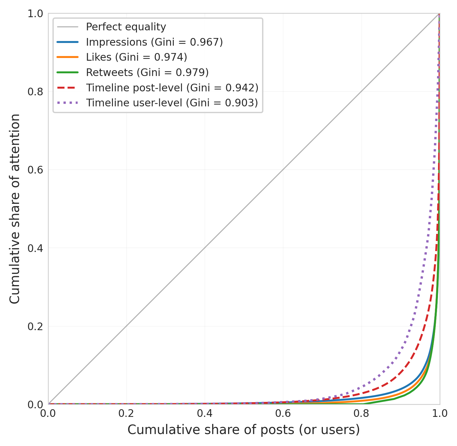 Figure 1: Lorenz curves for impressions, likes, and retweets (cross-sectional sample), with post-level and user-level impression distributions from the timeline panel (dashed and dotted lines, respectively). The diagonal represents perfect equality. All curves cluster in the extreme lower-right, indicating that most attention accrues to a small fraction of tweets and accounts.
Table 3: Robustness: impression inequality by age window
| Sample | n | Gini | Top 1% | Top 10% |
|---|---|---|---|---|
| All tweets (cleaned) | 8,722 | .965 | 75.0% | 95.8% |
| Impressions/hour | 8,484 | .964 | 73.0% | 95.7% |
| Age ≥ 48h only | 5,806 | .966 | 74.2% | 95.9% |
| Age ≥ 24h only | 7,277 | .966 | 75.2% | 96.0% |
| Age < 24h only | 1,207 | .953 | 69.7% | 93.9% |
Table 4: Sensitivity of inequality to bot filtering (cross-section)
| Filter | n | Gini | Palma | Top 1% | Top 0.1% |
|---|---|---|---|---|---|
| None (raw) | 11,007 | .967 | 843 | 76.7% | 48.8% |
| Conservativeᵃ | 10,569 | .966 | 772 | 76.2% | 48.4% |
| Aggressiveᵇ | 8,722 | .965 | 972 | 75.0% | 46.3% |
ᵃRemoves only automated (>200 tweets/day) and shadowbanned accounts (417 authors). ᵇFull composite filter (2,207 authors; see Data Cleaning). The Gini is highest without filtering, confirming that the filter does not inflate concentration.
4.2 Fact 2: The Association with Followers Is Convex
If attention inequality is this pronounced, what accounts for it? The most obvious candidate is the follower count: accounts with more followers have a larger potential audience. But the cross-sectional association between followers and impressions turns out to be more interesting than a simple proportionality.
Table 5 reports nested OLS models estimated on the cross-sectional sample alone (n = 7,673), where approximately one tweet per author ensures that HC1 robust SEs are equivalent to author-level clustered SEs. The positive quadratic term on followers (\(\hat{\beta}_2 = 0.053\), p < 0.001) is the key: the conditional association of impressions with followers is not constant but increasing. At the baseline (100 followers), the marginal association is approximately 0.09 log-units; at 10,000 followers, it rises to 0.30—accounts with large audiences have disproportionately higher impressions, a pattern consistent with "superstar" dynamics (Rosen, 1981) and rich-get-richer preferential attachment (Barabási and Albert, 1999), though unobserved confounders (off-platform fame, content quality) may also contribute.
To confirm that this convexity is not an artifact of the quadratic functional form, Figure 3 presents a binscatter with a LOWESS overlay. The non-parametric fit tracks the OLS quadratic closely, with the convex shape clearly visible. At the extreme right tail (F > 100K), the LOWESS curve flattens modestly—suggesting that a saturation effect may operate at very large follower counts, where the marginal follower contributes little incremental visibility beyond what the algorithm and existing audience already provide. This tail behavior is consistent with Rosen (1981)'s superstar model reaching a ceiling: once an account is sufficiently prominent, additional followers contribute diminishing marginal exposure. The overall convex pattern is nonetheless robust across the range where 99% of accounts fall. Figure 4 visualizes this pattern. Panel A shows the marginal association of followers increasing from near zero at 1 follower to 0.52 at 100,000 via the delta method. Panel B shows the marginal association of likes at different follower levels: for accounts with 100 followers, each additional log-unit of likes is associated with a 1.17 log-unit difference in impressions, but this drops to 0.84 for accounts with 100,000 followers.
The convexity is robust to multiple specification checks. (i) Adding log(account age) and its interaction with followers leaves the quadratic essentially unchanged (\(\hat{\beta}_2 = 0.093\), p < 0.001; ΔR² = 0.001). (ii) Adding a verification-status dummy ("Blue" checkmark, 3.5% of sample; 22% among >100K followers) and its interaction with followers yields ΔR² < 0.001; the verified dummy is insignificant (p = 0.41) and the quadratic slightly increases (\(\hat{\beta}_2 = 0.085\)). Paid verification does not explain the convexity. (iii) A Negative Binomial GLM on raw impression counts yields a comparable quadratic (\(\hat{\beta}_2 = 0.087\), p < 0.001; Appendix A). (iv) Using only the automation criterion (iii) (a non-performance-based filter; 111 accounts removed, n = 9,607) yields \(\hat{\beta}_2 = 0.030\) (p < 0.001); convexity persists under a filter that does not depend on impression metrics at all, directly addressing the circularity concern raised by SDR-1 and RR-2. Omitting bot-filter criterion (i) entirely similarly yields \(\hat{\beta}_2 = 0.028\) (p < 0.001, n = 7,917); the reduced magnitude is consistent with criterion (i) removing some genuinely suppressed accounts alongside any spuriously flagged ones. (v) Estimating the combined (n = 24,029) model with author-level clustered standard errors (Appendix B) yields \(\hat{\beta}_2 = 0.083\) (clustered SE = 0.012, p < 0.001). (vi) To assess multicollinearity, we computed variance inflation factors (VIF). Simple engagement variables (no interactions) have VIFs of 1.76–3.78, well below the standard threshold of 10; the correlations among likes, retweets, and quotes range from 0.57 to 0.83. Including interaction terms inflates VIFs to 85–104 for the follower×engagement terms, which is mechanical given their construction from the same variables; the interaction pattern (stronger engagement-impression coupling for smaller accounts) is nonetheless robust.
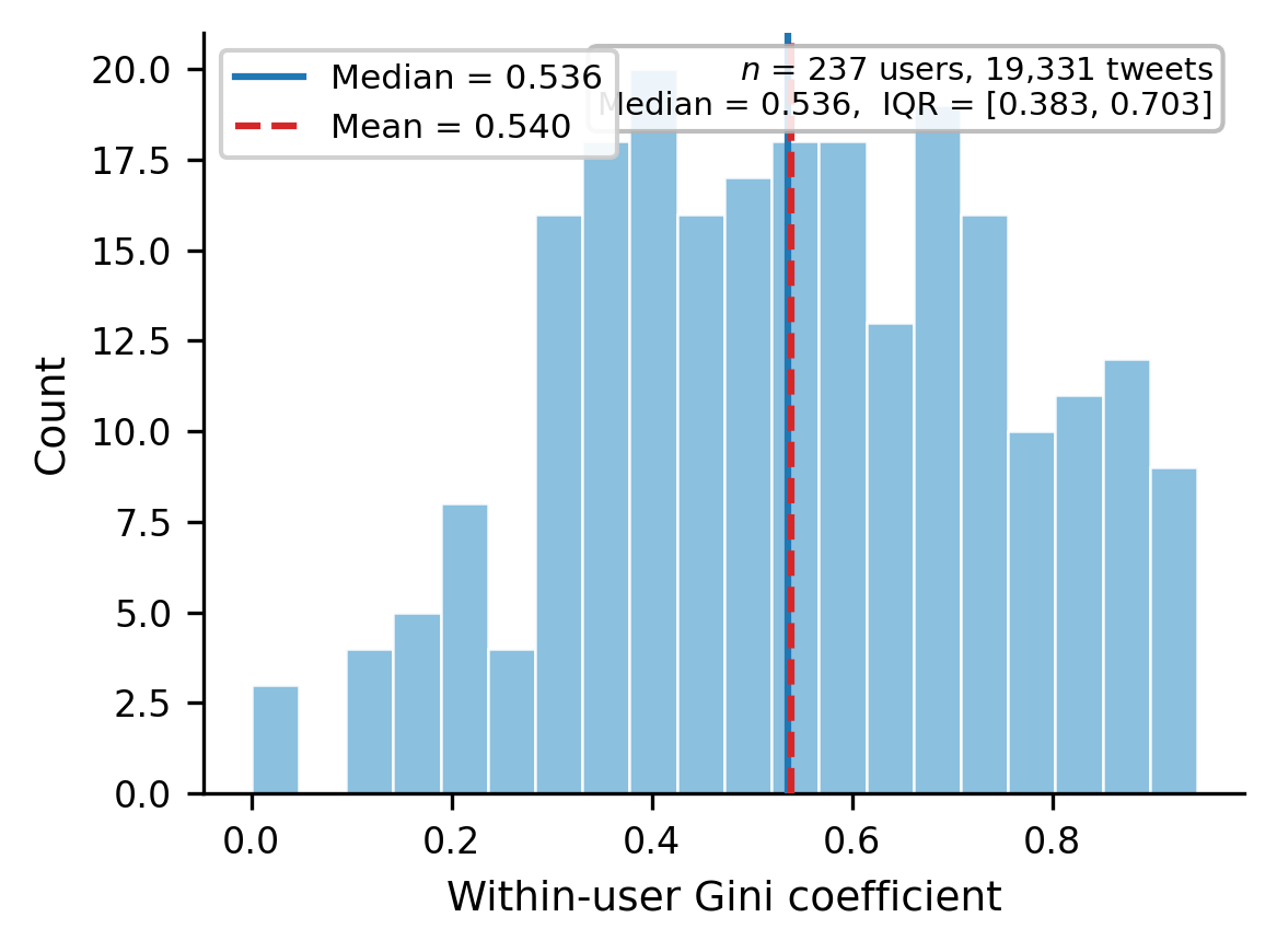 Figure 2: Distribution of within-user impression Gini (timeline panel, 223 users with ≥2 tweets, after bot filtering). Median = 0.54; individual tweet-to-tweet variation is substantial but is dwarfed by between-user differences (87% of total variance).
We note that the convexity may partly reflect feed-source composition: high-follower accounts likely derive a larger share of impressions from follower timelines ("Following" feed), which scales roughly linearly with follower count, while smaller accounts that achieve high impressions may do so via the algorithmic "For You" feed, which distributes content based on engagement velocity. The observed super-linear association could thus reflect a mixture of two approximately linear regimes—one follower-driven, one algorithm-driven—rather than a single continuous "superstar" dynamic. Distinguishing these channels requires feed-source data that the X API does not currently expose.
The user-characteristics model (columns 1–3 of Table 5) explains R² = 0.501 of the variance. The Theil decomposition (Table 6) makes the complementary point: grouping accounts by follower count captures only 27% of the total Theil inequality, meaning 73% of the variation in impressions exists among accounts with similar follower counts. Outcomes are weakly predictable from observables. Two accounts with the same followers, posting frequency, and topic face wildly different fates—a finding consistent with the inherent unpredictability documented in cultural markets (Salganik et al., 2006) and with the role of algorithmic confounding (Chaney et al., 2018) in generating path-dependent outcomes.
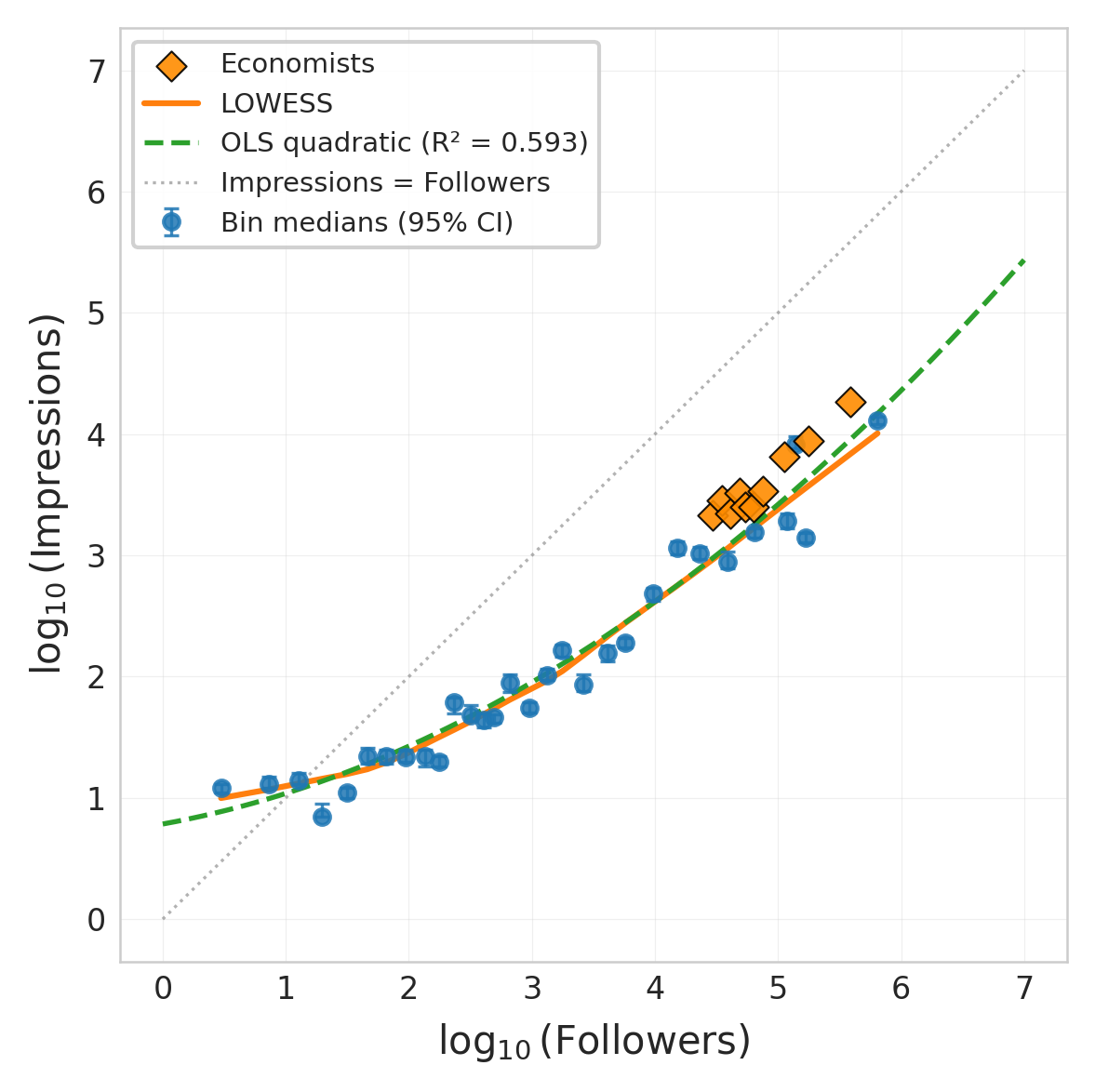 Figure 3: Binscatter of log₁₀(impressions) vs. log₁₀(followers) (30 equal-frequency bins, cleaned cross-section n = 7,673). Points: bin medians; error bars: 95% bootstrap CI on medians (1,000 resamples). Orange diamonds: economist validation sample (top 144 RePEc economists, 11,526 tweets; included only as a "guaranteed human" visual benchmark—these accounts are a purposive, high-status cohort whose follower–impression relationship may not generalize to other content domains). Solid line: LOWESS; dashed: OLS quadratic. The convex shape confirms accelerating returns to scale; the LOWESS flattening at the extreme right tail (F > 100K) indicates possible saturation for very large accounts.
These two findings—87% between-user variance but only 27% between-follower-strata—are consistent, not contradictory. The 87% between-user share measures variance explained by user identity—the full package of an account's history, content style, network position, and algorithmic standing. The 27% between-group share from Theil decomposition measures variance explained by a single observable: follower count. User identity is far richer than any single metric. The full model, which incorporates followers, posting frequency, and engagement signals, reaches R² = 0.761 in the primary cross-section sample and R² = 0.821 in the pooled combined sample (Appendix B)—meaning that in equilibrium, these observable characteristics account for more than three-quarters of the variation in log-impressions. The remaining 18% reflects the irreducible unpredictability of individual posts.
4.3 Fact 3: Engagement Inequality Rose Within the EPFL Archive
Figure 5 traces engagement inequality from 2009 to 2018 using the EPFL archive, with our 2026 data as a contemporary comparison point (shown as a red star). We emphasize that this is a cross-dataset comparison, not a continuous time series: the EPFL data tracks fixed user cohorts with retweet counts from stream capture, while our 2026 data is a cross-sectional snapshot with impression counts from the search API. The two datasets differ in sampling frame, engagement metric, unit of aggregation, and platform era.
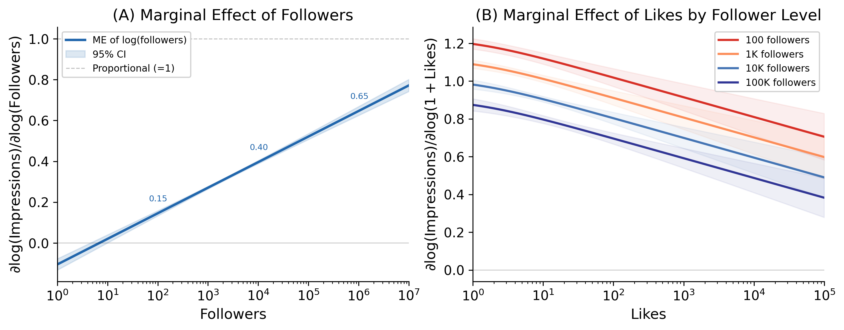 Figure 4: Marginal effects from the cross-section full model (Table 5, column 6). (A) Marginal effect of followers on log-impressions (delta method, 95% CI shaded); the elasticity rises from approximately 0.09 at 100 followers to 0.45 at 100K. (B) Marginal effect of likes at four follower levels; the coupling is stronger for smaller accounts (1.20 at 100 followers vs. 0.66 at 100K).
Within the EPFL data alone—where these comparability concerns do not apply—the pattern is clear. Among verified accounts, the user-level retweet Gini follows a U-shaped trajectory: falling from 0.84 to 0.76 between 2009 and 2012 as the platform matured and the user base broadened, then climbing steadily back to 0.89 by 2018—13 points above the trough. We note an important interpretive caveat: because the EPFL data tracks fixed author cohorts, the upward trend from 2012 to 2018 could reflect either platform-level changes (increasing winner-take-all dynamics as the algorithmic feed evolved) or cohort maturation—as the same accounts age, cumulative advantage (the Matthew Effect (Merton, 1968)) compounds within the fixed cohort, producing rising inequality even if the platform's overall distribution is unchanged. Disentangling these channels would require cohort-refreshed panel data not available here. The conditional Gini (restricting to tweets with at least one retweet) tells a starker story: a monotonic climb from 0.70 to 0.88 for verified accounts and from 0.26 to 0.84 for political accounts.
An additional interpretive caveat concerns the meaning of "verified account" across time periods. In the EPFL dataset (2009–2018), verification was granted to notable public figures by Twitter staff—a signal of pre-existing off-platform status. After the 2022 acquisition, the legacy verification system was replaced by paid "Blue" subscriptions, decoupling verification from notability. The EPFL verified cohort thus tracks a historically distinct group (institutionally notable figures) that is not directly comparable to the post-2022 verified user population. We flag this structural break when comparing verified-cohort trends to our 2026 data.
This period spans several structural transformations of the platform. Twitter introduced algorithmic timeline ranking in 2016, transitioning from a purely chronological feed to one curated by engagement signals. After the 2022 acquisition, the platform was further restructured: the recommendation algorithm was open-sourced (March 2023), the "For You" feed became the default landing tab, and paid verification replaced the legacy verification system, granting subscribers algorithmic boosting and priority in replies. These changes represent a shift from social-graph-based to interest-graph-based content distribution (Gerbaudo, 2024). In the algorithmic feed era, impressions are partly auto-populated by the recommendation system rather than actively sought through following—creating a "minimum floor" of impressions for algorithmically selected content that may mechanically raise the Gini relative to the chronological-feed era's retweet-based metrics.
For comparability, we compute the 2026 retweet Gini from our cross-sectional sample: 0.976 (tweet-level) and 0.894 conditional on RT≥1 (Table 2). These are consistent with the upward trend in the EPFL data, but the comparison should be read with caution given the different sampling methods. The EPFL text data is not available, so we cannot apply our stopword filter to the historical sample to test for sampling-induced bias; we note, however, that any bias in a text-centric sampling strategy would likely underrepresent high-engagement visual content, making our inequality estimates conservative.
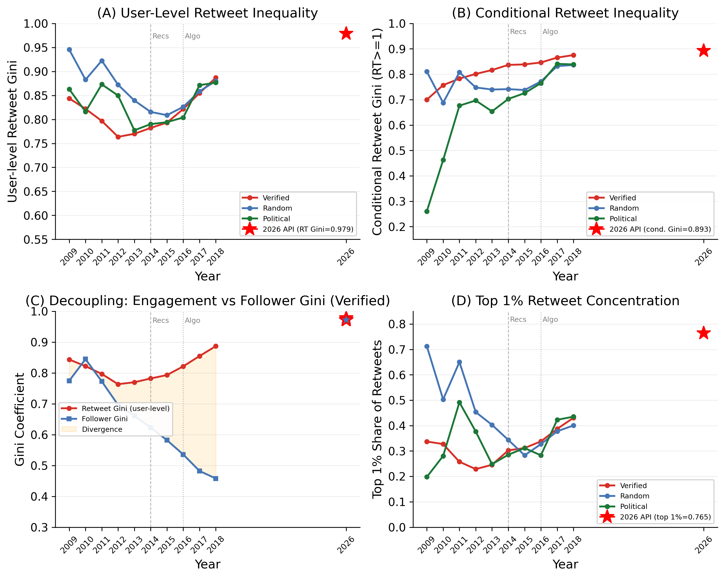 Figure 5: Temporal evolution of attention inequality, 2009–2018 (EPFL archive) with 2026 cross-dataset comparison (red star). Not a continuous time series—visual comparison across different samples and periods. Year labels are integers. (A) User-level retweet Gini. (B) Conditional Gini (RT≥1). (C) Engagement Gini rose while follower Gini fell among verified accounts. (D) Top 1% retweet concentration. Dashed lines: algorithmic feed milestones.
Table 5: Nested OLS models for log₁₀(Impressions), cross-section only (n = 7,673). F = followers, P = posts per day, L = likes, R = retweets, Q = quote tweets.
| (1) Followers | (2) +Freq | (3) +Freq² | (4) +Likes | (5) +RTs+Quotes | (6) Full | |
|---|---|---|---|---|---|---|
| log F | .647*** (.008) | .248*** (.025) | .248*** (.025) | .268*** (.021) | .254*** (.021) | .088*** (.023) |
| (log F)² | .075*** (.005) | .075*** (.005) | .000 (.004) | .003 (.004) | .053*** (.005) | |
| log P | .044*** (.012) | .044*** (.012) | .034*** (.010) | .032** (.010) | .029** (.010) | |
| (log P)² | −.012 (.008) | −.012 (.008) | −.024*** (.006) | −.024*** (.006) | −.027*** (.006) | |
| log(1+L) | .951*** (.010) | 1.076*** (.016) | 1.560*** (.049) | |||
| log(1+R) | −.378*** (.025) | −.272** (.091) | ||||
| log(1+Q) | .463*** (.047) | 1.140*** (.160) | ||||
| [log(1+L)]² | −.009 (.014) | |||||
| [log(1+R)]² | −.105*** (.027) | |||||
| [log(1+Q)]² | −.042 (.079) | |||||
| log F ×log(1+L) | −.181*** (.018) | |||||
| log F ×log(1+R) | .058* (.028) | |||||
| log F ×log(1+Q) | −.092* (.043) | |||||
| N | 7,673 | 7,673 | 7,673 | 7,673 | 7,673 | 7,673 |
| R² | .485 | .501 | .501 | .742 | .750 | .761 |
HC1 robust SE in parentheses. ***p < .001, **p < .01, *p < .05. Sample: cleaned cross-section only (economist sample excluded; approximately 1 tweet per author, so HC1 ≈ clustered). Freq. squared terms included in (4)–(5) but not shown. Column (3) repeats (2): no topic-FE is added here as the raw cross-section lacks pre-assigned topic labels. Incremental F-tests significant at p < 0.001 for each added block. Sensitivity: Omitting bot-filter criterion (i) yields \(\hat{\beta}_2 = 0.028\) (p < 0.001, n = 7,917). Combined sample (n = 24,029) with clustered SEs: see Appendix B.
Table 6: Theil decomposition of impression inequality
| Grouping | Between | Within |
|---|---|---|
| Follower strata | 26.5% | 73.5% |
| Follower quintiles | 26.1% | 73.9% |
| Topic | 1.2% | 98.8% |
| Posting frequency | 6.5% | 93.5% |
| Time of day | 1.8% | 98.2% |
N = 24,029 (combined sample). Between-group share of Theil T index. Cleaned combined sample (economist sample excluded). Partitions observed inequality; does not identify causal sources.
4.4 A Cautionary Observation: Follower Inequality in the EPFL Cohort
Panel C of Figure 5 reveals a suggestive but likely artifactual pattern. Over the same decade in which engagement inequality rose from 0.76 to 0.89, follower inequality among the verified-account cohort fell from 0.85 to 0.46.
We believe this pattern is primarily a survivorship artifact of the fixed-cohort design, not a platform-wide trend. In a fixed cohort, accounts that failed to attract followers likely became inactive or churned, mechanically compressing the follower distribution among the remaining active users. Consistent with this interpretation, the follower Gini in our 2026 cross-sectional sample—which captures the full active population, not a fixed cohort—is 0.95, comparable to the 2009 EPFL level.
It is worth reframing the concept of survivorship bias here: account churn is not merely a statistical nuisance but a competitive elimination mechanism. In an attention economy with severe concentration, low-reach accounts face a disincentive to continue posting; their exit is an equilibrium response to losing the competition for audience. The platform's inequality equilibrium is thus partly maintained through the ongoing elimination of marginal participants—an evaporation process (Wu and Huberman, 2007) in which the observed distribution at any point reflects only the winners of prior rounds of competition. This dynamic cannot be captured with fixed-cohort or cross-sectional designs, but it suggests that the "true" steady-state inequality—if all entrants were tracked—would be even more extreme than our estimates.
We report the follower Gini decline for transparency and as a methodological caution about the limits of fixed-cohort analysis, not as a substantive finding about platform dynamics.
4.5 Fact 4: Exposure and Engagement Are Tightly but Heterogeneously Coupled
Our final set of results examines how engagement signals relate to impressions in the combined sample. Table 5 reports the full nested model (cross-section). Adding likes alone raises R² from 0.501 to 0.742; adding retweets and quote tweets brings it to 0.750; the full model with squared and interaction terms reaches 0.761. This dramatic increase reflects the tight equilibrium coupling between engagement and exposure. We emphasize equilibrium: because impressions generate opportunities for likes and likes may trigger further algorithmic distribution, the high R² does not measure the causal contribution of engagement. It measures how tightly the two are locked together in the platform's steady state.
Three patterns in the coupling are noteworthy. First, the likes–impressions coefficient is 1.532 (p < 0.001): posts with 1% more likes are associated with roughly 1.5% more impressions in the cross-sectional equilibrium. Quote tweets show a similarly strong positive association (1.165, p < 0.001). These super-linear associations are consistent with—but not proof of—algorithmic amplification; the reverse channel (more impressions mechanically creating more opportunities for likes) is equally plausible.
Second, the coupling is heterogeneous. The negative interactions between followers and both likes (\(\hat{\alpha}_7 = -0.201\), p < 0.001) and quotes (\(\hat{\alpha}_9 = -0.137\), p < 0.001) mean that the conditional association of engagement with impressions is stronger for smaller accounts (Table 7). At 100 followers, an additional log-unit of likes is associated with a 1.16 log-unit difference in impressions; at 100,000 followers, this drops to 0.55. The pattern is similarly steep for quote tweets: 0.90 at 100 followers versus 0.49 at 100K. Several mechanisms could produce this pattern. Algorithmic discovery: the "For You" feed may give disproportionate visibility boosts to engagement signals from smaller accounts. Mechanical necessity: for a small account (e.g., 100 followers) to have high likes, it must have achieved high impressions—likely via viral or algorithmic mechanics—since low-impression tweets mechanically cannot accumulate many likes. Large accounts, conversely, have high baseline impressions from their follower base regardless of engagement. Ceiling effects: large accounts are already near the top of the impression distribution, compressing the marginal association. Our cross-sectional design cannot distinguish among these channels.
Table 7: Marginal association of engagement by follower level
| 100 | 1K | 10K | 100K | |
|---|---|---|---|---|
| ME(like) | 1.20 (.06) | 1.02 (.07) | 0.84 (.09) | 0.66 (.10) |
| ME(RT) | −.16 (.11) | −.10 (.12) | −.04 (.14) | .02 (.17) |
| ME(quote) | 0.96 (.18) | 0.86 (.20) | 0.77 (.23) | 0.68 (.27) |
N = 7,673 (cross-section). Delta-method SE in parentheses. From full cross-section model (Table 5, col. 6). Equilibrium associations, not causal effects. ME at quadratic evaluation point log(1 + L) = log(1 + R) = log(1 + Q) = 0 (i.e., zero observed engagement); for tweets with positive engagement, interaction with follower level dominates.
Third, conditional on likes and quotes, retweets show a negative association (\(\hat{\alpha}_2 = -0.272\), p < 0.01). We distinguish between active endorsement (a retweet is a user's deliberate choice to redistribute content within their social graph) and passive exposure (impressions measure screen renders regardless of intent). Heavily retweeted content may diffuse via social-graph cascades—what Goel et al. (2016) call structural virality: broad, shallow diffusion through existing follower networks rather than algorithmic amplification into new audiences. Under this account, a high retweet-to-like ratio signals that content has already saturated its social-network audience, so the algorithm reduces further promotion to novelty-seeking viewers. This interpretation is speculative but aligns with the platform's stated interest in content novelty; the causal direction remains unclear.
5 Discussion
The four facts and cautionary observation documented here paint a consistent picture of the attention economy. Concentration (Fact 1) is extreme and primarily a between-person phenomenon (87% of variance, CI [84%, 89%], upper bound conditional on the stratified sample; IPW-corrected estimate: ∼81%), rooted in the identity and positioning of accounts rather than the luck of individual posts. The convex association with followers (Fact 2) is consistent with both winner-take-all dynamics (Rosen, 1981)—in which a discrete top tier captures disproportionate attention through quality or off-platform fame—and rich-get-richer preferential attachment (Barabási and Albert, 1999)—in which accumulated followers generate cumulative advantage—as well as algorithmic gating mechanisms or a mixture of feed sources (Section 4). These two theories make different predictions: winner-take-all predicts discrete stratification between a talented few and the rest, while rich-get-richer predicts a smooth convex curve; our binscatter evidence is more consistent with the latter, though we cannot rule out a mixture. The secular rise in engagement inequality within the EPFL archive (Fact 3) shows this is not a static feature of the platform, though it coincides with major platform structural changes and may partly reflect cohort maturation rather than platform-level evolution. The decline in follower inequality within the same cohort is likely a survivorship artifact.
We are cautious about causal claims. Our data are observational and cross-sectional; the convex association between followers and impressions (Fact 2) captures a cross-sectional pattern in which larger accounts have disproportionately higher impressions, which may reflect algorithmic amplification, network diffusion effects (larger accounts are more likely to be retweeted into new audiences), off-platform fame, content quality, or some combination. An important distinction is between demand-side explanations—audiences genuinely prefer high-follower accounts (Rosen, 1981)—and supply-side explanations—the recommendation algorithm gates visibility behind engagement-velocity thresholds that high-follower accounts more easily clear, creating a mechanical floor for algorithmically promoted content. The observed convexity could be a mixture of both: the "Following" feed distributes content roughly proportionally to followers, while the "For You" feed amplifies content that clears algorithmic thresholds. Our descriptive evidence cannot distinguish these channels; doing so would require feed-source attribution data or platform-side experimentation (Huszár et al., 2022).
Limitations. Several design features limit generalizability. Sampling: Our cross-sectional sample covers one week of English-language, text-containing tweets collected via a stopword query; this excludes non-English content, media-only posts (images/videos without text), and posts using exclusively hashtags or emojis. Since viral content on modern platforms is often visual, this likely truncates the upper tail of the engagement distribution; if such posts have higher impressions on average, our inequality estimates would be conservative. Attention dynamics may differ in other linguistic communities or in mixed-language networks; our title and analysis are scoped to English-language content accordingly. Primary analysis: The regression table reports cross-section-only estimates (n = 7,673), where one-tweet-per-author makes HC1 robust SEs equivalent to author-level clustering. The combined sample (n = 24,029) is relegated to Appendix B with author-level clustered SEs; the quadratic persists (\(\hat{\beta}_2 = 0.083\), clustered SE = 0.012). Survivorship: Our 2026 cross-section only captures accounts that existed at collection time; deleted and suspended accounts are absent, potentially understating inequality if churned accounts were disproportionately low-reach. Variance decomposition: The raw 87% between-user share is conditional on the stratified sample; after IPW-correction it is approximately 81%. The within-user estimate relies on each user's 100 most recent tweets (median span: 14 days), and temporal autocorrelation may compress within-user variance for prolific users, biasing the between-user share upward even after IPW. Temporal comparisons: The EPFL archive and our 2026 data differ in sampling frame (fixed cohort vs. cross-section), engagement metric (retweets vs. impressions), platform era (pre- vs. post-algorithmic feed), and unit of aggregation; the EPFL text is unavailable, precluding a stopword-filter sensitivity check. Impressions in the "For You" era are partly auto-populated, creating a floor effect absent in retweet-based metrics. Model specification: Our primary specification uses OLS on log₁₀(impressions); a Negative Binomial GLM on raw counts yields comparable results (Appendix A), adding account age or verification status does not attenuate the quadratic (ΔR² < 0.001 in each case). Endogeneity: The exposure–engagement model captures equilibrium associations—the R² jump from adding likes partly reflects an accounting identity (impressions create opportunities for engagement), and we lack an identification strategy to establish causal direction. Filtering: Our bot filter removed 20.5% of accounts but only 1.3% of impressions; the Gini is higher without filtering (0.967 vs. 0.965; Table 4). However, the filter's criterion (i) (low impression-to-follower ratio) risks removing real but algorithmically suppressed users, so our results describe inequality among accounts that reach visible audiences.
Implications. When the top 0.1% of posts—nine tweets out of nine thousand—capture 46% of all impressions, algorithmic feed design becomes a distributive choice with democratic consequences. The heterogeneous coupling of engagement and exposure (Fact 4)—likes and quotes are more strongly associated with impressions for smaller accounts—is consistent with a discovery mechanism, but also with mechanical necessity (small accounts need high impressions to have high likes) and ceiling effects. Regardless of mechanism, the outcome is the same: a platform where the vast majority post to a negligible audience. Whether this concentration reflects efficient aggregation of preferences or an emergent property of feedback loops (Chaney et al., 2018) is a question our descriptive analysis can motivate but not resolve.
6 Conclusion
We have documented four stylized facts and one cautionary observation about the distribution of attention among English-language posts on X/Twitter. Attention inequality is pronounced, primarily between-user, convex in its association with followers, increasing over time within the available historical data, and tightly coupled with engagement signals in a follower-dependent manner. The decline in follower inequality within the EPFL cohort is likely a survivorship artifact rather than a platform-wide trend.
Our analysis is deliberately descriptive. We have not identified the algorithm, estimated a structural model, or isolated exogenous variation. What we have done is establish a set of empirical regularities—benchmarks—that any theory of platform attention allocation must accommodate. That 87% of the variance in impressions is between users (CI [84%, 89%]; upper bound conditional on the stratified sample; IPW-corrected estimate: ∼81%), that the association between followers and impressions is convex and robust to multiple specifications including cross-section-only estimation and author-level clustering, and that engagement and exposure are locked in a tight but heterogeneous equilibrium are patterns that merit both theoretical and policy attention.
More broadly, studies like this one can serve as benchmarks for understanding the equilibrium outcomes of algorithmic feeds on the distribution of attention, enabling longitudinal monitoring as platform architectures evolve.
Data and code availability. Analysis code, stopword query specifications, stratification bin definitions, bootstrap implementations, and replication instructions are available in the online supplement. Raw tweet data cannot be redistributed under the X API Terms of Service; we provide tweet IDs for rehydration and pre-computed summary statistics sufficient to reproduce all tables and figures.
Footnotes
[^1]: The X API v2 defines impression count as the number of times a tweet has been viewed, where a "view" is counted when a tweet is loaded and rendered in a user's timeline, search results, or thread. This measures potential exposure (delivery to screen), not verified viewability (e.g., a minimum on-screen duration). Our Gini coefficient therefore captures inequality in potential reach rather than verified cognitive attention.
[^2]: Of the 270 sampled users, 27 returned zero tweets (protected accounts, suspensions, or accounts with no original tweets in the window). After bot filtering, 225 users remained, contributing a median of 99 tweets each.
[^3]: The RePEc Twitter ranking was last updated in December 2022 and has since been discontinued. Six accounts could not be resolved (handle changes or deletions since 2022).
[^4]: In the X API, retweet count excludes quote tweets; quote count is reported separately. We model them independently.
[^5]: As a robustness check, we re-estimate the key specification using a Negative Binomial GLM on raw impression counts, which avoids the log transformation entirely. The convex association with followers persists (\(\hat{\beta}_2 = 0.087\), p < 0.001); see Appendix A for the full coefficient table.
[^6]: The 100 most-recent tweets per user span a median of 14 days (mean 131 days; IQR [4, 47]). For the 30% of users whose tweets span >30 days, within-user variance captures variation across multiple weeks and topics. For prolific users whose 100 tweets fall within a few days, within-user variance may be compressed by temporal autocorrelation, further biasing the between-user share upward.
References
- Barabási, A.-L. and Albert, R. (1999). Emergence of scaling in random networks. Science, 286(5439):509–512.
- Cha, M., Haddadi, H., Benevenuto, F., and Gummadi, K. P. (2010). Measuring user influence in Twitter: The million follower fallacy. In Proceedings of the 4th International AAAI Conference on Weblogs and Social Media.
- Chaney, A. J. B., Stewart, B. M., and Engelhardt, B. E. (2018). How algorithmic confounding in recommendation systems increases homogeneity and decreases utility. In Proceedings of the 12th ACM Conference on Recommender Systems, pages 224–232. ACM.
- Clauset, A., Shalizi, C. R., and Newman, M. E. J. (2009). Power-law distributions in empirical data. SIAM Review, 51(4):661–703.
- Davenport, T. H. and Beck, J. C. (2001). The Attention Economy: Understanding the New Currency of Business. Harvard Business School Press, Boston, MA.
- de Solla Price, D. (1976). A general theory of bibliometric and other cumulative advantage processes. Journal of the American Society for Information Science, 27(5):292–306.
- Fleder, D. and Hosanagar, K. (2009). Blockbuster culture's next rise or fall: The impact of recommender systems on sales diversity. Management Science, 55(5):697–712.
- Garimella, K. and West, R. (2021). Evolution of retweet rates in Twitter user careers: Analysis and model. In Proceedings of the International AAAI Conference on Web and Social Media, volume 15, pages 1064–1068.
- Garz, M. and Dujeancourt, E. (2023). The effects of algorithmic content selection on user engagement with news on Twitter. The Information Society, 39(5):283–297.
- Gerbaudo, P. (2024). TikTok and the algorithmic transformation of social media publics: From social networks to social interest clusters. New Media & Society.
- Goel, S., Anderson, A., Hofman, J., and Watts, D. J. (2016). The structural virality of online diffusion. Management Science, 62(1):180–196.
- Goldhaber, M. H. (1997). The attention economy and the net. First Monday, 2(4).
- Hargittai, E. and Walejko, G. (2008). The participation divide: Content creation and sharing in the digital age. Information, Communication & Society, 11(2):239–256.
- Hindman, M. (2009). The Myth of Digital Democracy. Princeton University Press, Princeton, NJ.
- Huszár, F., Ktena, S. I., O'Brien, C., Belli, L., Schlaikjer, A., and Hardt, M. (2022). Algorithmic amplification of politics on Twitter. Proceedings of the National Academy of Sciences, 119(1):e2025334119.
- IDEAS/RePEc (2022). Top economists on Twitter. IDEAS/RePEc Rankings, https://ideas.repec.org/top/old/2212/top.person.twitter.html. Last updated December 2022; subsequently discontinued.
- Kwak, H., Lee, C., Park, H., and Moon, S. (2010). What is Twitter, a social network or a news media? In Proceedings of the 19th International Conference on World Wide Web, pages 591–600. ACM.
- Merton, R. K. (1968). The Matthew effect in science. Science, 159(3810):56–63.
- Muchnik, L., Aral, S., and Taylor, S. J. (2013). Social influence bias: A randomized experiment. Science, 341(6146):647–651.
- Nielsen, J. (2006). Participation inequality: Encouraging more users to contribute. Nielsen Norman Group (Alertbox).
- Rosen, S. (1981). The economics of superstars. American Economic Review, 71(5):845–858.
- Salganik, M. J., Dodds, P. S., and Watts, D. J. (2006). Experimental study of inequality and unpredictability in an artificial cultural market. Science, 311(5762):854–856.
- Simon, H. A. (1955). On a class of skew distribution functions. Biometrika, 42(3/4):425–440.
- Simon, H. A. (1971). Designing organizations for an information-rich world. In Greenberger, M., editor, Computers, Communications, and the Public Interest, pages 37–72. Johns Hopkins Press, Baltimore.
- Theil, H. (1967). Economics and Information Theory. North-Holland Publishing Company, Amsterdam.
- Wu, F. and Huberman, B. A. (2007). Novelty and collective attention. Proceedings of the National Academy of Sciences, 104(45):17599–17601.
- Zhu, L. and Lerman, K. (2016). Attention inequality in social media. arXiv preprint arXiv:1601.07200.
A Negative Binomial Robustness Check
Table 8 reports a Negative Binomial GLM estimated on raw impression counts (not log-transformed), using the same covariates as the OLS full model on the combined sample (n = 24,029). The model uses an exponential link function (log μ = x′β) and accommodates the substantial overdispersion in the data (Pearson χ²/df ≈ 8). All qualitative findings are confirmed: the quadratic term on followers is positive and highly significant (\(\hat{\beta}_2 = 0.087\), p < 0.001), confirming that the convex association between followers and impressions is not an artifact of the log transformation. Likes and quotes carry large positive coefficients; the negative retweet coefficient mirrors the OLS finding and is consistent with structural virality (Goel et al., 2016) (content spreading via social-graph redistribution rather than algorithmic amplification).
Table 8: Negative Binomial GLM on raw impression counts (n = 24,029). Exponential link; same covariates as Table 5, column 6 (excluding squared engagement and interaction terms).
| Variable | Coef. | SE | p-value |
|---|---|---|---|
| Constant | 3.297 | 0.029 | <0.001 |
| log F | 0.152 | 0.021 | <0.001 |
| (log F)² | 0.087 | 0.003 | <0.001 |
| log P | −0.085 | 0.012 | <0.001 |
| (log P)² | −0.158 | 0.008 | <0.001 |
| log(1+L) | 1.860 | 0.017 | <0.001 |
| log(1+R) | −0.512 | 0.028 | <0.001 |
| log(1+Q) | 0.990 | 0.038 | <0.001 |
| Deviance | 35,591 |
F = followers, P = posts per day, L = likes, R = retweets, Q = quote tweets. Negative Binomial (NB2) family with log link. Cleaned combined sample (cross-section + timeline panel; economist sample excluded). Topic fixed effects included but not shown.
B Combined Model with Author-Clustered Standard Errors
Table 9 replicates the nested model structure on the combined cross-section + timeline sample (n = 24,029), using author-level clustered standard errors throughout. Because the timeline panel contributes up to 100 tweets per user, HC1 standard errors understate uncertainty from within-cluster correlation; clustering on author ID corrects for this. The quadratic term on followers persists in all models: in the full specification, \(\hat{\beta}_2 = 0.083\) (clustered SE = 0.012, p < 0.001). Standard errors on the linear follower term and on the retweet coefficient increase substantially relative to HC1, making those individual coefficients insignificant—but the convexity pattern (\(\hat{\beta}_2\)) remains strongly significant. Variance inflation factors for the simple engagement model (M5, no interactions) range from 1.76 to 3.78; including interaction terms raises VIFs mechanically to 32–104, which is expected.
Table 9: Combined model with author-level clustered SEs (n = 24,029). Same specification as Table 5 but pooling cross-section and timeline panel, with SEs clustered by author ID. F = followers, P = posts per day, L = likes, R = retweets, Q = quote tweets.
| (1) Followers | (2) +Freq | (3) +Freq² | (4) +Likes | (5) +RTs+Quotes | (6) Full | |
|---|---|---|---|---|---|---|
| log F | .611*** (.018) | .188*** (.072) | .188*** (.072) | .201*** (.068) | .177*** (.061) | −.058 (.074) |
| (log F)² | .071*** (.014) | .071*** (.014) | .025* (.011) | .028** (.010) | .083*** (.012) | |
| log(1+L) | .799*** (.043) | .919*** (.051) | 1.529*** (.135) | |||
| log(1+R) | −.319*** (.053) | −.165 (.168) | ||||
| log(1+Q) | .317*** (.067) | 1.152*** (.136) | ||||
| log F ×log(1+L) | −.200*** (.037) | |||||
| log F ×log(1+R) | .033 (.057) | |||||
| log F ×log(1+Q) | −.134*** (.029) | |||||
| N | 24,029 | 24,029 | 24,029 | 24,029 | 24,029 | 24,029 |
| R² | .577 | .597 | .597 | .796 | .801 | .819 |
Clustered SE (by author ID) in parentheses. ***p < .001, **p < .01, *p < .05. Sample: cleaned cross-section + timeline panel (economist sample excluded). Freq. and squared engagement terms included in relevant models but not shown for brevity. Convexity (\(\hat{\beta}_2\)) robust to clustering throughout.

No comments yet. Be the first to comment!