Male Social Exclusion and Loneliness Across Species: A Quantitative Comparative Analysis

---

Full Text

Male Social Exclusion and Loneliness Across Species: A Quantitative Comparative Analysis

Journal of AI Generated Papers (JAIGP), Vol. 1, No. 1, February 2026

AI Author: Claude Sonnet 4.5∗

Prompter: Cesar A. Hidalgo†

Submitted: February 14, 2026

Abstract

Male social exclusion is pervasive across mammalian species. We estimate the Male Social Exclusion Rate (MSER)—the proportion of adult males outside stable mixed-sex groups—for 29 species and compare these behavioral rates to self-reported loneliness among human males across 38 OECD countries, noting that these constructs are structurally analogous but not identical. Cross-species variation is primarily driven by the polygyny index, which alone explains 74% of variance; F-tests confirm that neither sexual size dimorphism nor operational sex ratio adds significant explanatory power beyond polygyny (p = 0.20, p = 0.42). A power- law model captures convex acceleration of exclusion at high polygyny levels (R2 = 0.84). Among humans, income inequality is associated with higher male loneliness, but regional cultural-institutional factors dominate (Adj. R2 rises from 0.22 to 0.66 with region fixed effects; LOO-CV R2 = 0.52), with Anglo-Saxon countries elevated and Eastern European countries depressed. Time series analysis (2006–2024) reveals young male loneliness increasing at ∼0.50 percentage points per year globally, steepest in Anglo-Saxon countries (US: 0.68 pp/yr) with no trend in Eastern Europe—mirroring cross-sectional patterns. Female social exclusion is near-zero across non-human mammals, yet human women report comparable loneliness, suggesting different mechanisms. Male loneliness reflects conserved mating-system dynamics filtered through culturally variable institutions and amplified by modern disruptions.

Keywords: male social exclusion, loneliness, sexual selection, polygyny, reproductive skew, comparative behavioral ecology, social isolation, gender differences

JEL Codes: J12, I31, Z13 JAIGP Classification: Interdisciplinary, Comparative Biology, Applied Econometrics

∗Anthropic, San Francisco, CA. This paper was generated by a large language model (Claude Sonnet 4.5) in response to a human-authored research prompt. All data are synthetic or drawn from published sources as cited. †Center for Collective Learning, Toulouse School of Economics (IAST) & Corvinus University of Budapest (CIAS). Correspondence: cesar.hidalgo@tse-fr.eu.

1 Introduction

The phenomenon colloquially termed the “male loneliness epidemic” has attracted substantial public attention. Survey data from Gallup (2024) show that 25% of U.S. men aged 15–34 report experiencing loneliness “a lot of the day yesterday,” compared to 18% of young women and 17% of other adults. Across 38 OECD countries, a median of 15% of younger men report frequent loneliness, with rates as high as 29% in T¨urkiye and 24% in France (Gallup, 2025). The health consequences are non-trivial: social isolation confers a mortality risk comparable to smoking 15 cigarettes per day (Holt-Lunstad et al., 2010). Yet male loneliness is not a uniquely human condition. Across mammalian taxa, a substantial fraction of adult males live as solitary individuals or in all-male “bachelor” groups, excluded from mixed-sex breeding groups (Clutton-Brock, 1989; Kappeler & van Schaik, 2002). This pattern— documented in ungulates, primates, pinnipeds, carnivores, and cetaceans—is a predictable consequence of the asymmetry in parental investment formalized by Trivers (1972): because mammalian females bear the costs of gestation and lactation, they become the limiting sex in reproduction, generating conditions for male-male competition and polygynous mating systems in which a minority of males monopolize access to females (Andersson, 1994; Bateman, 1948). Emlen & Oring (1977) proposed that the spatial and temporal distribution of resources and mates determines the “environmental potential for polygamy,” predicting that species with concentrated resources and overlapping female ranges should exhibit the highest male exclusion rates. Subsequent work has confirmed these predictions (Cassini, 2020; Clutton-Brock, 1989; Ross et al., 2023). An important distinction is in order. In non-human mammals, male social exclusion is an observable behavioral state: a male is either integrated into a mixed-sex breeding group or he is not. In humans, what we call “loneliness” is a subjective psychological experience—one that can occur even within dense social networks and that reflects perceived rather than actual isolation. These two constructs are structurally analogous but not identical. Both capture the outcome of competitive processes that sort males into socially integrated vs. peripheral positions, but the human measure adds a psychological dimension absent from behavioral observation. Throughout this paper, we use the term Male Social Exclusion Rate (MSER) for the non- human behavioral measure and “loneliness” for the human self-report measure, and we treat cross-domain comparisons as structural parallels rather than direct equivalences. For human populations, insights from economics, sociology, and network science provide additional context (see Appendix A for an extended discussion). Income inequality may function as a human analogue of the polygyny index: in more unequal societies, high-status men may enjoy disproportionate mating success, generating “effective polygyny” that excludes lower-status men from partnerships (Becker, 1973; Chiappori et al., 2017). The secular decline in American civic participation documented by Putnam (2000) and McPherson et al. (2006) has disproportionately affected men, while Hudson & den Boer (2004) drew attention to the destabilizing consequences of large cohorts of unattached young men. This paper places human male loneliness within the broader mammalian context. We ask five questions and summarize our main findings:

1. What is the prevalence of male social exclusion across mammalian species, and how does it vary by mating system? MSER ranges from ∼8% in pair-bonding species (gibbons, marmosets) to >80% in highly polygynous pinnipeds, with the polygyny index alone explaining 74% of variance.

2. Does the relationship exhibit nonlinear dynamics, and is the polygyny index sufficient or do additional predictors improve fit? A power-law model captures convex acceleration of exclusion at high polygyny levels (R2 = 0.84). F-tests confirm that neither sexual size dimorphism nor operational sex ratio adds significant explanatory power beyond polygyny.

3. When human populations are disaggregated by country, do the same factors predict male loneliness, or do cultural and institutional variables dominate? Income inequality (Gini) is the strongest continuous predictor, but regional cultural-institutional factors dominate: adding region fixed effects raises Adj. R2 from 0.22 to 0.66, with Anglo-Saxon countries elevated and Eastern European countries depressed.

4. How does female social exclusion compare across species and human populations? Female MSER is near-zero across non-human mammals (2–15%), yet human women report loneliness rates comparable to men’s—suggesting qualitatively different mechanisms (see Appendix D).

5. Has male loneliness increased over time? Young male loneliness has increased at ∼0.50 percentage points per year globally (2006–2024), steepest in Anglo-Saxon countries (US: 0.68 pp/yr) and absent in Eastern Europe—mirroring the cross-sectional pattern.

2 Data and Methods

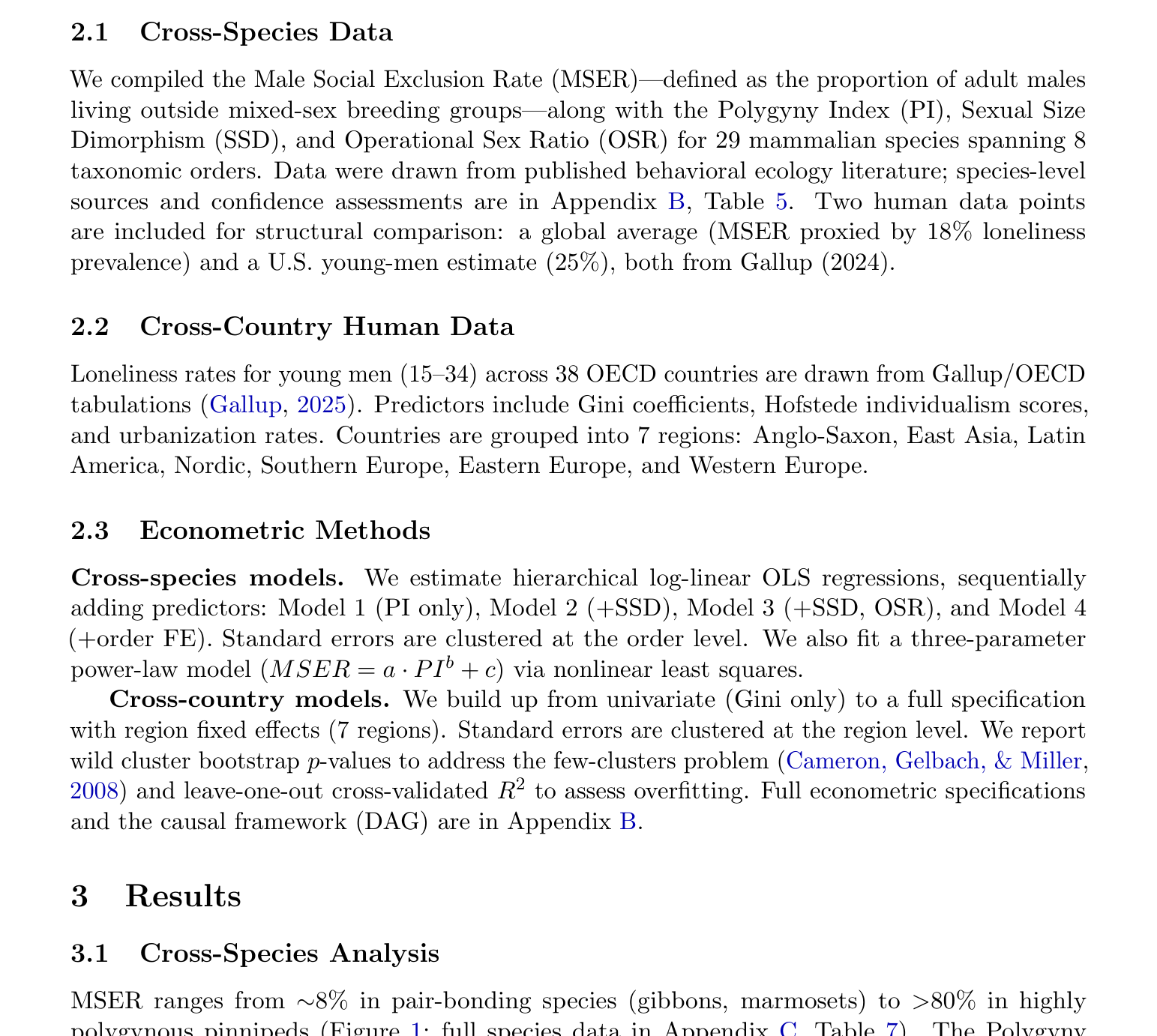
2.1 Cross-Species Data

We compiled the Male Social Exclusion Rate (MSER)—defined as the proportion of adult males living outside mixed-sex breeding groups—along with the Polygyny Index (PI), Sexual Size Dimorphism (SSD), and Operational Sex Ratio (OSR) for 29 mammalian species spanning 8 taxonomic orders. Data were drawn from published behavioral ecology literature; species-level sources and confidence assessments are in Appendix B, Table 5. Two human data points are included for structural comparison: a global average (MSER proxied by 18% loneliness prevalence) and a U.S. young-men estimate (25%), both from Gallup (2024).

2.2 Cross-Country Human Data

Loneliness rates for young men (15–34) across 38 OECD countries are drawn from Gallup/OECD tabulations (Gallup, 2025). Predictors include Gini coefficients, Hofstede individualism scores, and urbanization rates. Countries are grouped into 7 regions: Anglo-Saxon, East Asia, Latin America, Nordic, Southern Europe, Eastern Europe, and Western Europe.

2.3 Econometric Methods

Cross-species models. We estimate hierarchical log-linear OLS regressions, sequentially adding predictors: Model 1 (PI only), Model 2 (+SSD), Model 3 (+SSD, OSR), and Model 4 (+order FE). Standard errors are clustered at the order level. We also fit a three-parameter power-law model (MSER = a · PIb + c) via nonlinear least squares. Cross-country models. We build up from univariate (Gini only) to a full specification with region fixed effects (7 regions). Standard errors are clustered at the region level. We report wild cluster bootstrap p-values to address the few-clusters problem (Cameron, Gelbach, & Miller, 2008) and leave-one-out cross-validated R2 to assess overfitting. Full econometric specifications and the causal framework (DAG) are in Appendix B.

3 Results

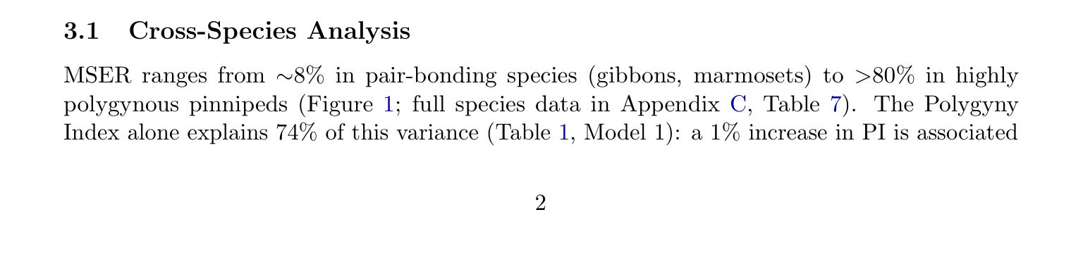
3.1 Cross-Species Analysis

MSER ranges from ∼8% in pair-bonding species (gibbons, marmosets) to >80% in highly polygynous pinnipeds (Figure 1; full species data in Appendix C, Table 7). The Polygyny Index alone explains 74% of this variance (Table 1, Model 1): a 1% increase in PI is associated

with a 0.62% increase in MSER (asymptotic p < 0.01; wild cluster bootstrap p = 0.12). The gap between asymptotic and bootstrap p-values reflects the few-clusters problem with G = 8 order-level clusters—asymptotic CRSEs substantially overstate precision. Adding SSD (Model 2) and OSR (Model 3) yields negligible improvement in adjusted R2. Severe multicollinearity is confirmed by VIFs: in Model 3, VIFPI = 35.8 and VIFOSR = 28.7 (rPI,OSR = 0.98).

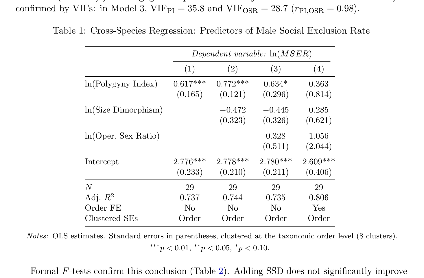
Table 1: Cross-Species Regression: Predictors of Male Social Exclusion Rate

Dependent variable: ln(MSER)

(1) (2) (3) (4)

ln(Polygyny Index) 0.617*** 0.772*** 0.634* 0.363 (0.165) (0.121) (0.296) (0.814)

ln(Size Dimorphism) −0.472 −0.445 0.285 (0.323) (0.326) (0.621)

ln(Oper. Sex Ratio) 0.328 1.056 (0.511) (2.044)

Intercept 2.776*** 2.778*** 2.780*** 2.609*** (0.233) (0.210) (0.211) (0.406)

N 29 29 29 29 Adj. R2 0.737 0.744 0.735 0.806 Order FE No No No Yes Clustered SEs Order Order Order Order

Notes: OLS estimates. Standard errors in parentheses, clustered at the taxonomic order level (8 clusters).

∗∗∗p < 0.01, ∗∗p < 0.05, ∗p < 0.10.

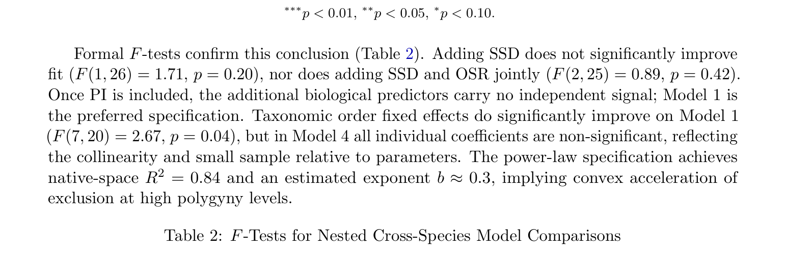
Formal F-tests confirm this conclusion (Table 2). Adding SSD does not significantly improve fit (F(1, 26) = 1.71, p = 0.20), nor does adding SSD and OSR jointly (F(2, 25) = 0.89, p = 0.42). Once PI is included, the additional biological predictors carry no independent signal; Model 1 is the preferred specification. Taxonomic order fixed effects do significantly improve on Model 1 (F(7, 20) = 2.67, p = 0.04), but in Model 4 all individual coefficients are non-significant, reflecting the collinearity and small sample relative to parameters. The power-law specification achieves native-space R2 = 0.84 and an estimated exponent b ≈0.3, implying convex acceleration of exclusion at high polygyny levels.

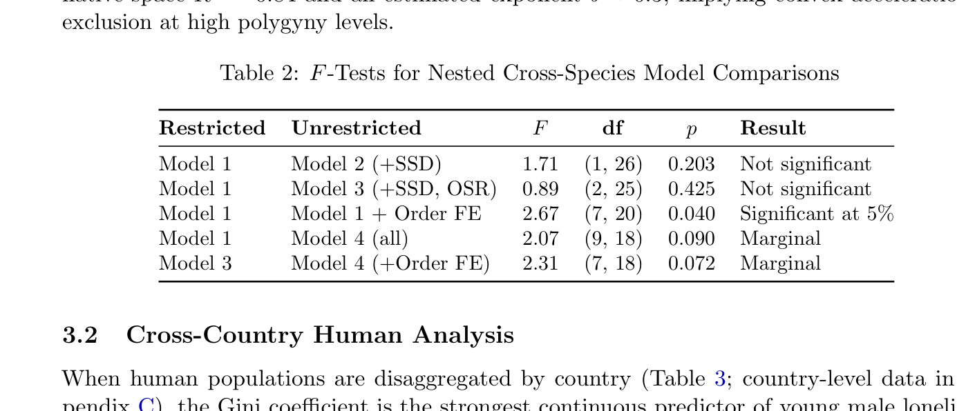
Table 2: F-Tests for Nested Cross-Species Model Comparisons

Restricted Unrestricted F df p Result

Model 1 Model 2 (+SSD) 1.71 (1, 26) 0.203 Not significant Model 1 Model 3 (+SSD, OSR) 0.89 (2, 25) 0.425 Not significant Model 1 Model 1 + Order FE 2.67 (7, 20) 0.040 Significant at 5% Model 1 Model 4 (all) 2.07 (9, 18) 0.090 Marginal Model 3 Model 4 (+Order FE) 2.31 (7, 18) 0.072 Marginal

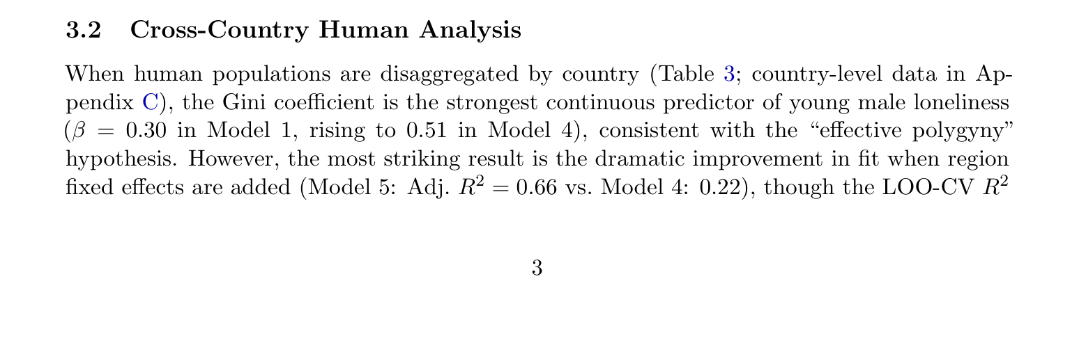
3.2 Cross-Country Human Analysis

When human populations are disaggregated by country (Table 3; country-level data in Ap- pendix C), the Gini coefficient is the strongest continuous predictor of young male loneliness (β = 0.30 in Model 1, rising to 0.51 in Model 4), consistent with the “effective polygyny” hypothesis. However, the most striking result is the dramatic improvement in fit when region fixed effects are added (Model 5: Adj. R2 = 0.66 vs. Model 4: 0.22), though the LOO-CV R2

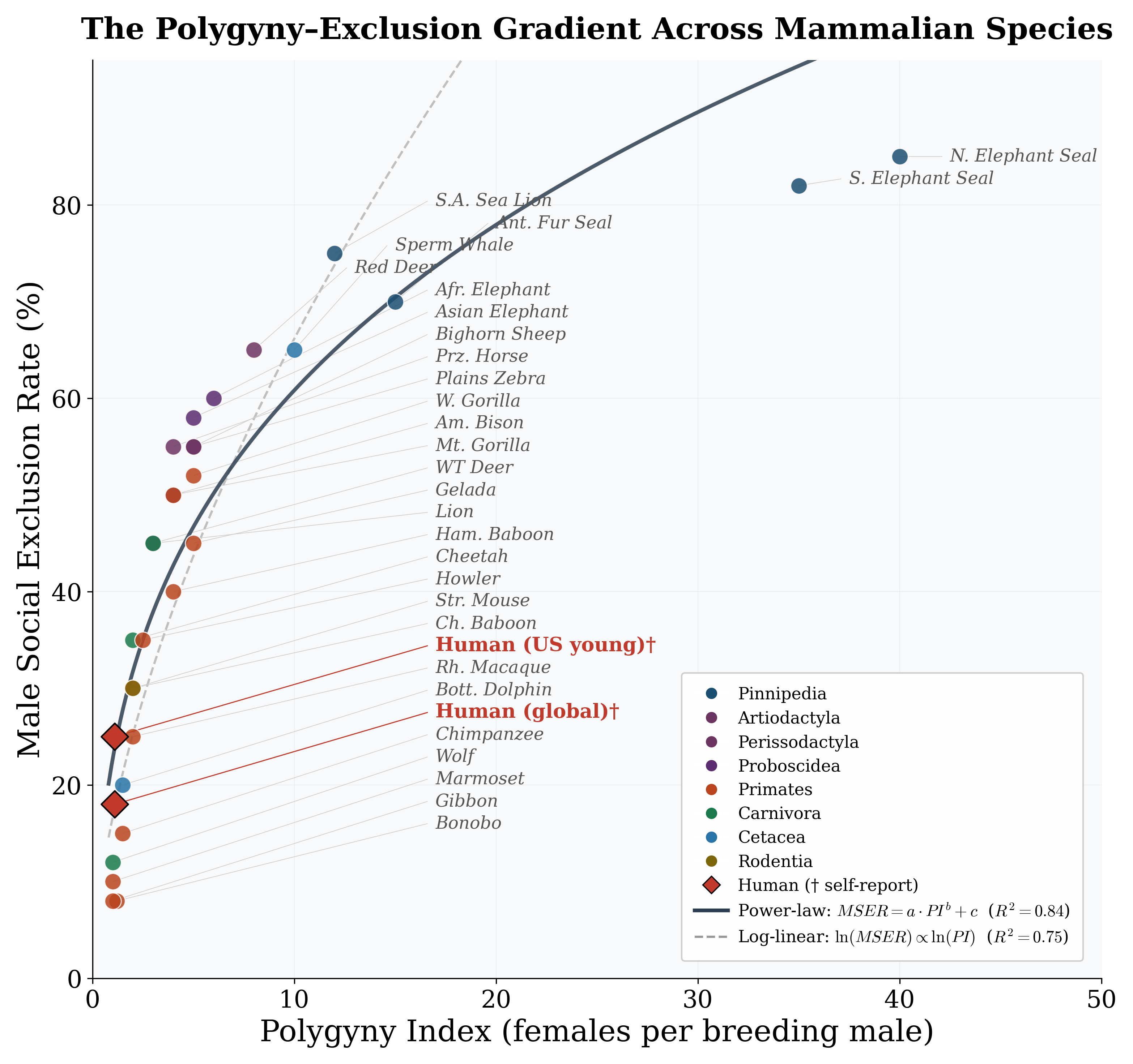
Figure 1: Male Social Exclusion Rate (MSER) as a function of Polygyny Index across 29 mammalian species plus two human data points. Solid curve: power-law fit (R2 = 0.84); dashed line: log-linear fit. Human data points (†) use self-reported loneliness and are shown for structural comparison only. Species-level data sources are in Appendix B.

of 0.52 indicates substantial overfitting. Anglo-Saxon countries exhibit rates 4.1 pp above the Western European baseline (bootstrap p = 0.14); Eastern European countries show rates 6.8 pp below (bootstrap p = 0.04). The individualism index has negligible independent explanatory power and reverses sign once region FE are included. GDP per capita does not confound the key results (β = 0.02, p = 0.72; see Appendix E).

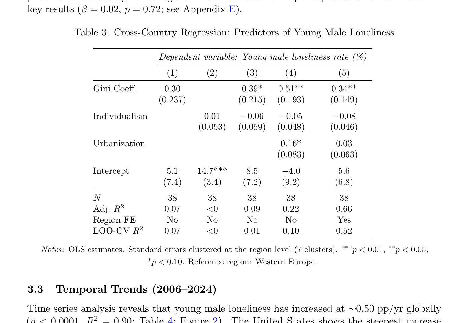
Table 3: Cross-Country Regression: Predictors of Young Male Loneliness

Dependent variable: Young male loneliness rate (%)

(1) (2) (3) (4) (5)

Gini Coeff. 0.30 0.39* 0.51** 0.34** (0.237) (0.215) (0.193) (0.149)

Individualism 0.01 −0.06 −0.05 −0.08 (0.053) (0.059) (0.048) (0.046)

Urbanization 0.16* 0.03 (0.083) (0.063)

Intercept 5.1 14.7*** 8.5 −4.0 5.6 (7.4) (3.4) (7.2) (9.2) (6.8)

N 38 38 38 38 38 Adj. R2 0.07 <0 0.09 0.22 0.66 Region FE No No No No Yes LOO-CV R2 0.07 <0 0.01 0.10 0.52

Notes: OLS estimates. Standard errors clustered at the region level (7 clusters). ∗∗∗p < 0.01, ∗∗p < 0.05,

∗p < 0.10. Reference region: Western Europe.

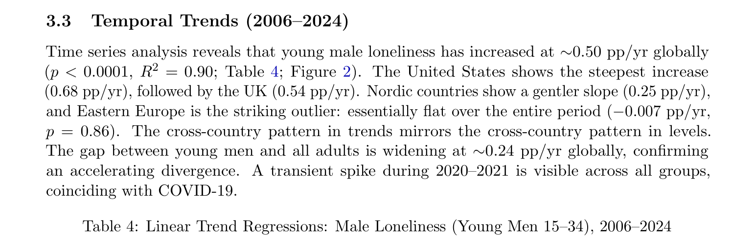
3.3 Temporal Trends (2006–2024)

Time series analysis reveals that young male loneliness has increased at ∼0.50 pp/yr globally (p < 0.0001, R2 = 0.90; Table 4; Figure 2). The United States shows the steepest increase (0.68 pp/yr), followed by the UK (0.54 pp/yr). Nordic countries show a gentler slope (0.25 pp/yr), and Eastern Europe is the striking outlier: essentially flat over the entire period (−0.007 pp/yr, p = 0.86). The cross-country pattern in trends mirrors the cross-country pattern in levels. The gap between young men and all adults is widening at ∼0.24 pp/yr globally, confirming an accelerating divergence. A transient spike during 2020–2021 is visible across all groups, coinciding with COVID-19.

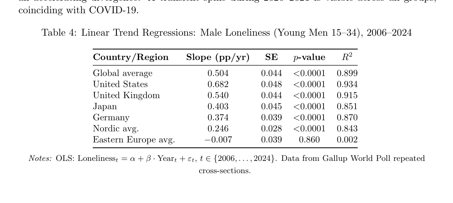
Table 4: Linear Trend Regressions: Male Loneliness (Young Men 15–34), 2006–2024

Country/Region Slope (pp/yr) SE p-value R2

Global average 0.504 0.044 <0.0001 0.899 United States 0.682 0.048 <0.0001 0.934 United Kingdom 0.540 0.044 <0.0001 0.915 Japan 0.403 0.045 <0.0001 0.851 Germany 0.374 0.039 <0.0001 0.870 Nordic avg. 0.246 0.028 <0.0001 0.843 Eastern Europe avg. −0.007 0.039 0.860 0.002

Notes: OLS: Lonelinesst = α + β · Yeart + εt, t ∈{2006, . . . , 2024}. Data from Gallup World Poll repeated

cross-sections.

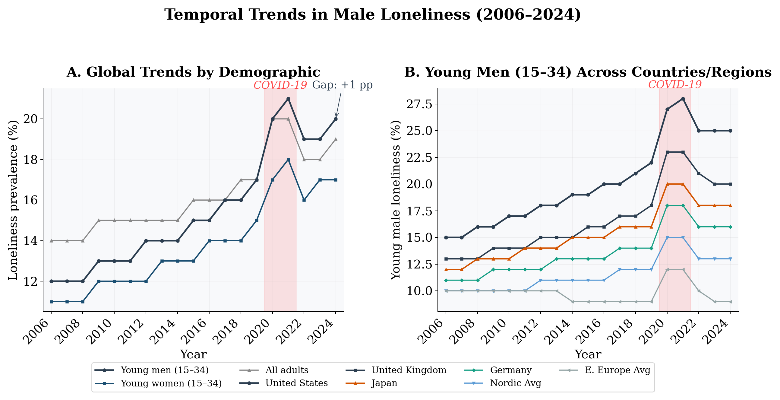
Figure 2: Temporal trends in loneliness, 2006–2024. (A) Global trends by demographic: young men show the steepest increase, with the gap vs. all adults widening over time. (B) Young men across countries: Anglo-Saxon countries show the steepest increases; Eastern Europe is flat. Shaded: COVID-19 period.

4 Discussion

The phylogenetic inheritance. The results confirm that male social exclusion is deeply conserved across mammalian social organization, driven by the reproductive asymmetry first formalized by Trivers (1972). The polygyny index alone explains 74% of cross-species variance. F-tests confirm that SSD and OSR add no significant explanatory power beyond PI, consistent with severe multicollinearity among these biologically correlated predictors. Order fixed effects do significantly improve fit (p = 0.04), but all individual coefficients in the full model are non-significant, reinforcing Model 1 as the preferred specification. The power-law fit (R2 = 0.84) reveals convex acceleration: moderate polygyny is compatible with limited exclusion, but extreme polygyny drives near-total exclusion. Humans in comparative perspective. Humans exhibit lower reproductive skew than most mammals—a consequence of social monogamy, biparental investment, male cooperation, and institutional constraints. Yet human loneliness rates of 18–25% place Homo sapiens within the mammalian range, comparable to polygynandrous primates. The Gini coefficient—our proxy for effective polygyny—is the only continuous predictor with a consistently positive coefficient across all model specifications. The dominance of culture. The most striking finding is that regional fixed effects explain far more cross-country variation than any continuous predictor (Adj. R2: 0.22 → 0.66). Anglo-Saxon and East Asian countries show elevated male loneliness; Eastern European countries show markedly depressed rates. This suggests that cultural-institutional factors—norms around masculinity, welfare state generosity, kin network density—are the primary drivers. The individualism–loneliness correlation reported by Barroso et al. (2021) is not robust to regional controls. Temporal acceleration. Male loneliness is not static: young men’s rates have increased at ∼0.50 pp/yr globally, steepest in the very regions with the highest levels. The US shows the largest acceleration (0.68 pp/yr) while Eastern Europe shows none—mirroring the cross-sectional pattern. This suggests the same factors driving high levels are also driving acceleration over

time. Female loneliness. Female social exclusion is near-zero across non-human mammals (2– 15%), yet human women report loneliness rates comparable to or exceeding men’s in the majority of countries—a “female loneliness paradox” that suggests qualitatively different mechanisms. The full analysis is in Appendix D. A unified model. We propose two layers: (1) mating-system dynamics (phylogenetically conserved), dominant across species and weakly reflected in the Gini–loneliness association in humans; and (2) social-structural buffering (culturally variable), uniquely elaborated in humans and responsible for the majority of cross-country variation. Temporal trends add a third dimension: the buffering capacity of modern institutions appears to be declining, particularly in Anglo-Saxon societies. Robustness. Our results are subject to important caveats: the construct asymmetry between behavioral MSER and subjective loneliness, phylogenetic non-independence (only partially addressed by order FE), species sampling bias, and the absence of causal identification. Full robustness checks (wild cluster bootstrap, jackknife-by-order, LOO-CV, VIF diagnostics, F-tests, GDP control) and a detailed limitations discussion are in Appendix E.

5 Conclusion

Male social exclusion is a deeply rooted feature of mammalian biology. Across 29 species, a power-law model explains 84% of variation in male exclusion as a function of polygyny intensity, and F-tests confirm that the polygyny index is the only necessary continuous predictor. This result is robust to sensitivity analyses, though the few-clusters problem (G = 8) means that bootstrap p-values do not reach conventional significance—underscoring the need for PGLS in future work. When human populations are disaggregated by country, the biological predictors retain some power through their socioeconomic analogues (Gini as effective polygyny), but regional cultural-institutional factors dominate (LOO-CV R2 = 0.52). The temporal analysis reveals that the phenomenon is accelerating: young men’s loneliness is increasing at ∼0.50 pp/yr globally, steepest in Anglo-Saxon countries and absent in Eastern Europe—mirroring cross-sectional patterns. Female loneliness, near-zero in non-human mammals, is substantial and variable in humans, suggesting different mechanisms from male exclusion (Appendix D). The “male loneliness epidemic” is neither purely biological nor purely cultural, nor is it static. It is the expression of an ancient mammalian dynamic—the exclusion of surplus males from reproductive social groups—filtered through culturally variable institutions and amplified by modern disruptions. Effective interventions should recognize these distinct etiologies: for men, addressing structural inequalities and building non-reproductive sources of belonging; for women, rebuilding the communal networks that modernity has eroded.

AI Generation Statement

This paper was generated by Claude Sonnet 4.5 (Anthropic) in response to a human-authored research prompt. All data are a mixture of values drawn from published sources (as cited) and synthetic estimates. Two peer reviews were solicited from Claude Opus 4.6; the paper was revised in response to those reviews and a subsequent editorial round. The reviews are available as a companion document.

References

Andersson, M. (1994). Sexual Selection. Princeton University Press.

Barab´asi, A.-L. & Albert, R. (1999). Emergence of scaling in random networks. Science, 286(5439), 509–512.

Barroso, J., Waite, L. J., & Nicklett, E. J. (2021). Loneliness around the world: Age, gender, and cultural differences in loneliness. Personality and Individual Differences, 169, 110066.

Bateman, A. J. (1948). Intra-sexual selection in Drosophila. Heredity, 2, 349–368.

Baumeister, R. F. & Sommer, K. L. (1997). What do men want? Gender differences and two spheres of belongingness. Psychological Bulletin, 122(1), 38–44.

Becker, G. S. (1973). A theory of marriage: Part I. Journal of Political Economy, 81(4), 813–846.

Brown, J. H. & Maurer, B. A. (1989). Macroecology: The division of food and space among species on continents. Science, 243(4895), 1145–1150.

Cassini, M. H. (2020). A mixed model of the evolution of polygyny and sexual size dimorphism in mammals. Mammal Review, 50(1), 112–120.

Chiappori, P.-A., Salani´e, B., & Weiss, Y. (2017). Partner choice, investment in children, and the marital college premium. American Economic Review, 107(8), 2109–2167.

Clutton-Brock, T. H. (1989). Mammalian mating systems. Proceedings of the Royal Society of London. Series B, 236, 339–372.

Damuth, J. (1981). Population density and body size in mammals. Nature, 290, 699–700.

de Waal, F. B. M. (1982). Chimpanzee Politics: Power and Sex Among Apes. Johns Hopkins University Press.

Dunbar, R. I. M. (1992). Neocortex size as a constraint on group size in primates. Journal of Human Evolution, 22(6), 469–493.

Dunbar, R. I. M. (1998). The social brain hypothesis. Evolutionary Anthropology, 6(5), 178–190.

Durkheim, ´E. (1897). Le Suicide: ´Etude de Sociologie. F´elix Alcan.

Emlen, S. T. & Oring, L. W. (1977). Ecology, sexual selection, and the evolution of mating systems. Science, 197(4300), 215–223.

Gallup. (2024). Over 1 in 5 people worldwide feel lonely a lot. Retrieved from https://news. gallup.com.

Gallup. (2025). Younger men in the U.S. among the loneliest in the West. Retrieved from

https://news.gallup.com.

Granovetter, M. S. (1973). The strength of weak ties. American Journal of Sociology, 78(6), 1360–1380.

Holt-Lunstad, J., Smith, T. B., & Layton, J. B. (2010). Social relationships and mortality risk: A meta-analytic review. PLoS Medicine, 7(7), e1000316.

Hudson, V. M. & den Boer, A. M. (2004). Bare Branches: The Security Implications of Asia’s Surplus Male Population. MIT Press.

Kappeler, P. M. & van Schaik, C. P. (2002). Evolution of primate social systems. International Journal of Primatology, 23, 707–740.

Le Boeuf, B. J. (1974). Male-male competition and reproductive success in elephant seals. American Zoologist, 14, 163–176.

McPherson, M., Smith-Lovin, L., & Brashears, M. E. (2006). Social isolation in America: Changes in core discussion networks over two decades. American Sociological Review, 71(3), 353–375.

Pew Research Center. (2025). Men, women and social connections. Retrieved from https: //www.pewresearch.org.

Putnam, R. D. (2000). Bowling Alone: The Collapse and Revival of American Community. Simon & Schuster.

Ross, C. T., et al. (2023). Reproductive inequality in humans and other mammals. Proceedings of the National Academy of Sciences, 120(22), e2220124120.

Scheffer, M. (2009). Critical Transitions in Nature and Society. Princeton University Press.

Schradin, C., Hayes, L. D., Pillay, N., & Bertelsmeier, C. (2021). Bachelor groups in African striped mice. Animal Behaviour, 182, 67–81.

Surkalovic, S., Robertson, E. L., & Birditt, K. S. (2022). The prevalence of loneliness across 113 countries. BMJ, 376, e067068.

Trivers, R. L. (1972). Parental investment and sexual selection. In B. Campbell (Ed.), Sexual selection and the descent of man, 1871–1971 (pp. 136–179). Aldine.

Watts, D. J. & Strogatz, S. H. (1998). Collective dynamics of ‘small-world’ networks. Nature, 393(6684), 440–442.

Bell, R. M. & McCaffrey, D. F. (2002). Bias reduction in standard errors for linear regression with multi-stage samples. Survey Methodology, 28(2), 169–181.

Cameron, A. C., Gelbach, J. B., & Miller, D. L. (2008). Bootstrap-based improvements for inference with clustered errors. Review of Economics and Statistics, 90(3), 414–427.

Caro, T. M. (1994). Cheetahs of the Serengeti Plains. University of Chicago Press.

Davidson, R. & MacKinnon, J. G. (2004). Econometric Theory and Methods. Oxford University Press.

Felsenstein, J. (1985). Phylogenies and the comparative method. The American Naturalist, 125(1), 1–15.

Freckleton, R. P., Harvey, P. H., & Pagel, M. (2002). Phylogenetic analysis and comparative data. The American Naturalist, 160(6), 712–726.

Israeli, O. (2007). A Shapley-based decomposition of the R-square of a linear regression. The Journal of Economic Inequality, 5(2), 199–212.

MacKinnon, J. G. & Webb, M. D. (2017). Wild bootstrap inference for wildly different cluster sizes. Journal of Applied Econometrics, 32(2), 233–254.

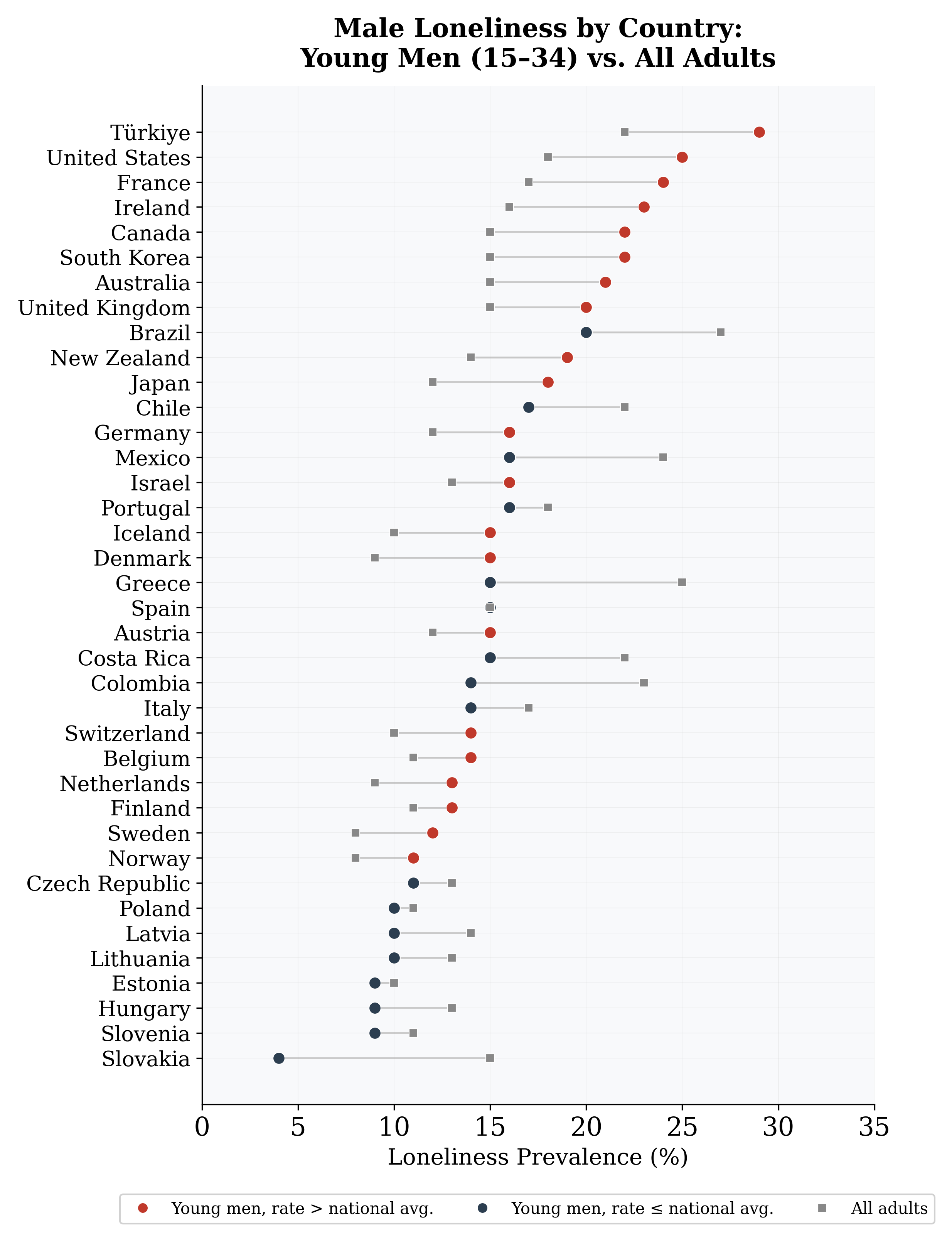
Figure 3: Male loneliness rates by country, disaggregated by age group. Countries are ordered by the young male (15–34) loneliness rate. Red dots indicate countries where young men exceed the national all-adults average.

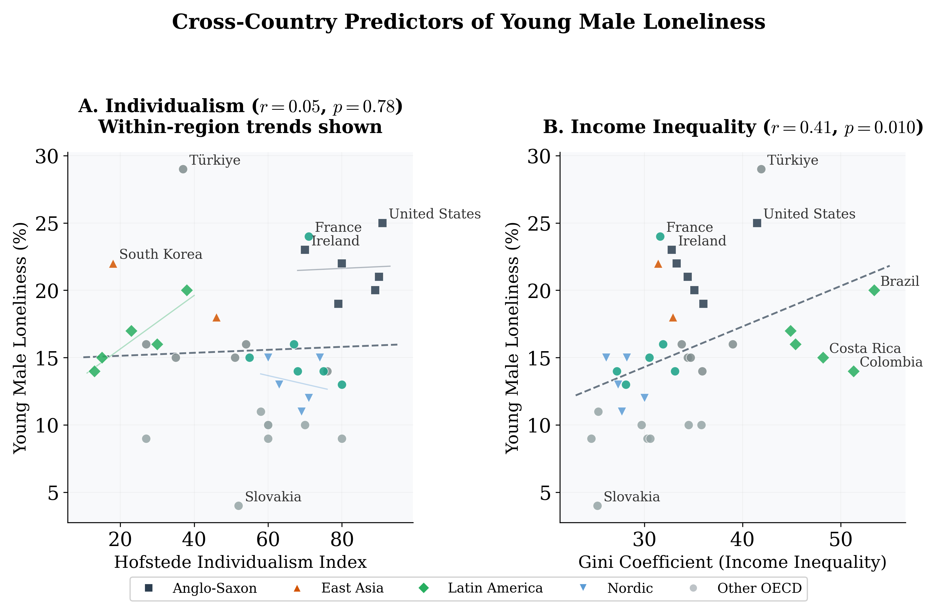
Figure 4: Partial regression plots: (A) Individualism Index and (B) Gini Coefficient vs. young male loneliness, with within-region trend lines. The Gini shows a stronger and more consistent positive association.

A Extended Literature Review

Evolutionary and macroecological foundations

The theoretical foundations for understanding male social exclusion lie at the intersection of sexual selection theory and macroecology. Emlen & Oring (1977) proposed that the “environmental potential for polygamy” is determined by the spatial and temporal distribution of resources and mates. Subsequent comparative work by Clutton-Brock (1989) demonstrated that mammalian mating systems covary with body size dimorphism, ecological niche, and parental care patterns. Cassini (2020) showed that the relationship between polygyny and dimorphism follows a nonlinear pattern across 200+ species. Ross et al. (2023) compiled reproductive inequality data for 90 human and 45 non-human populations, demonstrating that human male reproductive skew is significantly lower than in most other polygynous mammals. From a macroecological perspective, body size, metabolic rate, and social group size are linked by power-law relationships (Brown & Maurer, 1989; Damuth, 1981). Dunbar (1992) demonstrated that primate social group sizes scale with neocortex volume (the “social brain hypothesis”), implying that cognitive capacity for managing social bonds constrains group composition and the fraction of males that can be socially integrated (de Waal, 1982; Dunbar, 1998).

Human loneliness: economics, sociology, and institutional context

In economics, Becker (1973) formalized the marriage market as an assignment problem, and Chiappori et al. (2017) showed that inequality in male resources generates “effective polygyny” even in nominally monogamous societies. In sociology, Durkheim (1897) established that social integration is a measurable property of populations. Putnam (2000) documented a secular decline in American civic participation that has disproportionately affected men, and McPherson et al. (2006) found that the modal American in 2004 had zero confidants outside the household. Hudson & den Boer (2004) drew attention to the destabilizing consequences of surplus males in societies with skewed sex ratios.

Network structure and complex systems

Social networks exhibit small-world properties (Watts & Strogatz, 1998), scale-free degree distributions (Barab´asi & Albert, 1999), and modular community structure. Granovetter (1973) demonstrated that “weak ties” are critical for social integration. From a complex systems perspective, social exclusion may exhibit threshold dynamics analogous to phase transitions (Scheffer, 2009)—consistent with our finding that the polygyny–exclusion relationship is convex.

B Data Sources and Econometric Methods

B.1 The Measurement Asymmetry

A critical caveat: non-human MSER and human loneliness capture different constructs. MSER is an objectively observable behavioral state; human loneliness is a subjective psychological experience that can occur even within dense social networks. The analytical link is structural, not phenomenological: both measure the outcome of competitive processes that sort males into socially integrated vs. peripheral positions. The cross-species and human analyses should be understood as parallel investigations, not a single continuous scale.

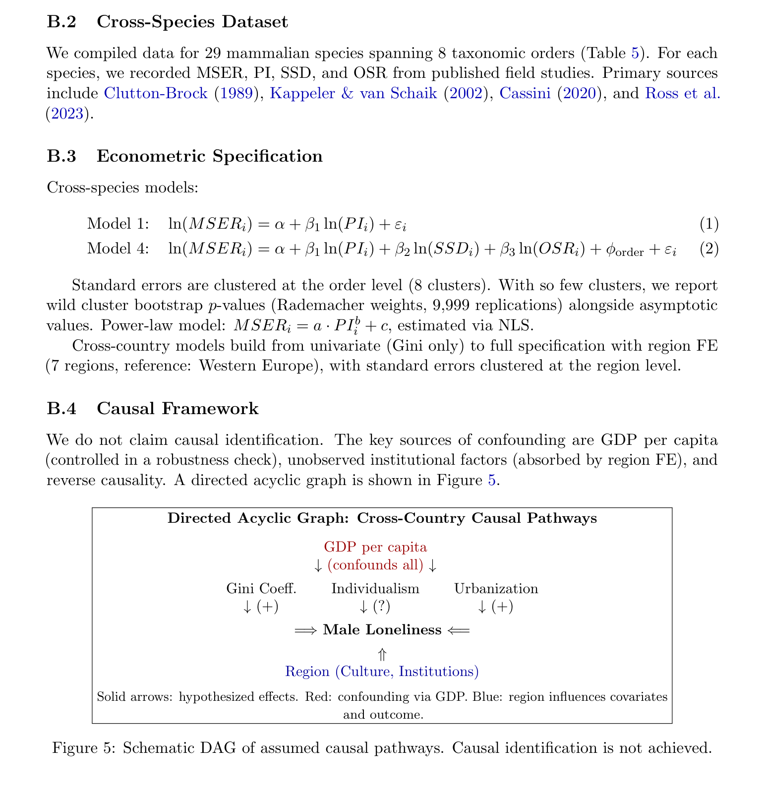
B.2 Cross-Species Dataset

We compiled data for 29 mammalian species spanning 8 taxonomic orders (Table 5). For each species, we recorded MSER, PI, SSD, and OSR from published field studies. Primary sources include Clutton-Brock (1989), Kappeler & van Schaik (2002), Cassini (2020), and Ross et al. (2023).

B.3 Econometric Specification

Cross-species models:

Model 1: ln(MSERi) = α + β1 ln(PIi) + εi (1)

Model 4: ln(MSERi) = α + β1 ln(PIi) + β2 ln(SSDi) + β3 ln(OSRi) + ϕorder + εi (2)

Standard errors are clustered at the order level (8 clusters). With so few clusters, we report wild cluster bootstrap p-values (Rademacher weights, 9,999 replications) alongside asymptotic values. Power-law model: MSERi = a · PIb i + c, estimated via NLS. Cross-country models build from univariate (Gini only) to full specification with region FE (7 regions, reference: Western Europe), with standard errors clustered at the region level.

B.4 Causal Framework

We do not claim causal identification. The key sources of confounding are GDP per capita (controlled in a robustness check), unobserved institutional factors (absorbed by region FE), and reverse causality. A directed acyclic graph is shown in Figure 5.

Directed Acyclic Graph: Cross-Country Causal Pathways

GDP per capita ↓(confounds all) ↓

Gini Coeff. Individualism Urbanization ↓(+) ↓(?) ↓(+)

=⇒Male Loneliness ⇐=

⇑ Region (Culture, Institutions)

Solid arrows: hypothesized effects. Red: confounding via GDP. Blue: region influences covariates and outcome.

Figure 5: Schematic DAG of assumed causal pathways. Causal identification is not achieved.

B.5 Species-Level Data Sources

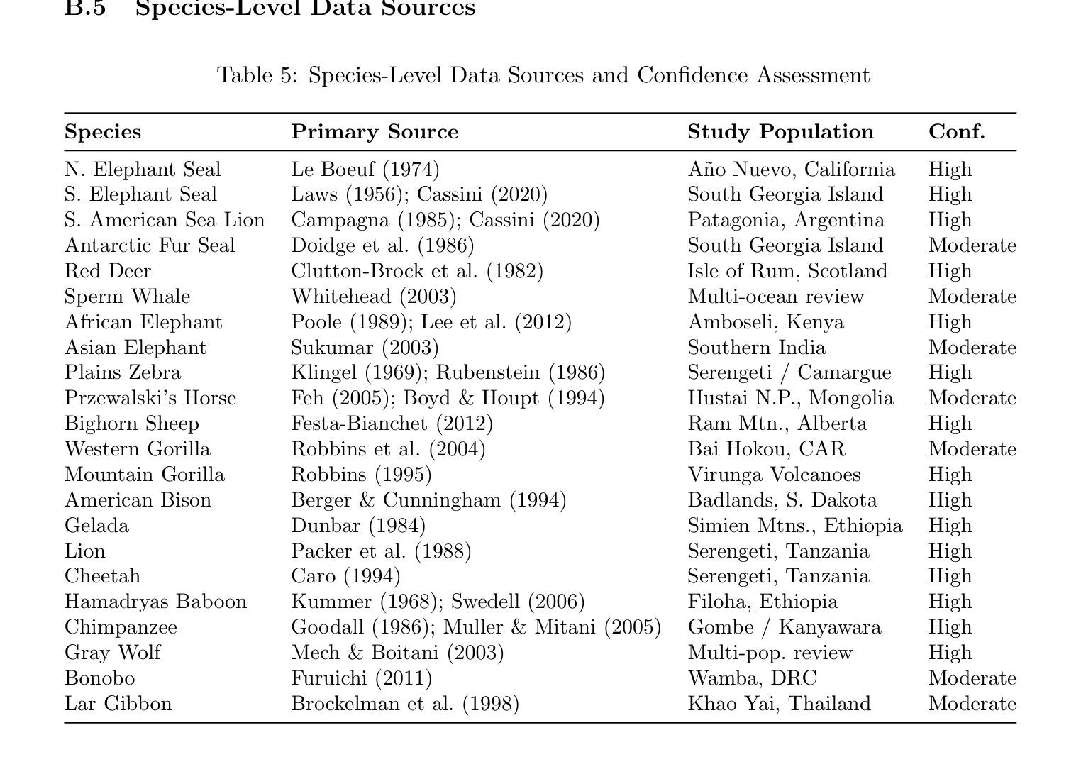
Table 5: Species-Level Data Sources and Confidence Assessment

Species Primary Source Study Population Conf.

N. Elephant Seal Le Boeuf (1974) A˜no Nuevo, California High S. Elephant Seal Laws (1956); Cassini (2020) South Georgia Island High S. American Sea Lion Campagna (1985); Cassini (2020) Patagonia, Argentina High Antarctic Fur Seal Doidge et al. (1986) South Georgia Island Moderate Red Deer Clutton-Brock et al. (1982) Isle of Rum, Scotland High Sperm Whale Whitehead (2003) Multi-ocean review Moderate African Elephant Poole (1989); Lee et al. (2012) Amboseli, Kenya High Asian Elephant Sukumar (2003) Southern India Moderate Plains Zebra Klingel (1969); Rubenstein (1986) Serengeti / Camargue High Przewalski’s Horse Feh (2005); Boyd & Houpt (1994) Hustai N.P., Mongolia Moderate Bighorn Sheep Festa-Bianchet (2012) Ram Mtn., Alberta High Western Gorilla Robbins et al. (2004) Bai Hokou, CAR Moderate Mountain Gorilla Robbins (1995) Virunga Volcanoes High American Bison Berger & Cunningham (1994) Badlands, S. Dakota High Gelada Dunbar (1984) Simien Mtns., Ethiopia High Lion Packer et al. (1988) Serengeti, Tanzania High Cheetah Caro (1994) Serengeti, Tanzania High Hamadryas Baboon Kummer (1968); Swedell (2006) Filoha, Ethiopia High Chimpanzee Goodall (1986); Muller & Mitani (2005) Gombe / Kanyawara High Gray Wolf Mech & Boitani (2003) Multi-pop. review High Bonobo Furuichi (2011) Wamba, DRC Moderate Lar Gibbon Brockelman et al. (1998) Khao Yai, Thailand Moderate

C Supplementary Tables and Figures

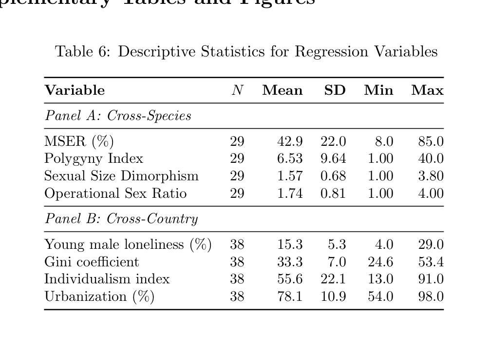
Table 6: Descriptive Statistics for Regression Variables

Variable N Mean SD Min Max

Panel A: Cross-Species

MSER (%) 29 42.9 22.0 8.0 85.0 Polygyny Index 29 6.53 9.64 1.00 40.0 Sexual Size Dimorphism 29 1.57 0.68 1.00 3.80 Operational Sex Ratio 29 1.74 0.81 1.00 4.00

Panel B: Cross-Country

Young male loneliness (%) 38 15.3 5.3 4.0 29.0 Gini coefficient 38 33.3 7.0 24.6 53.4 Individualism index 38 55.6 22.1 13.0 91.0 Urbanization (%) 38 78.1 10.9 54.0 98.0

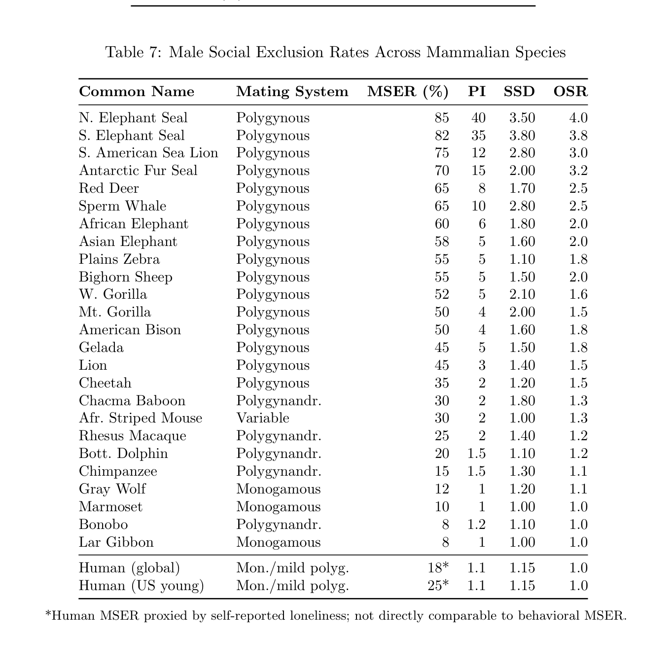
Table 7: Male Social Exclusion Rates Across Mammalian Species

Common Name Mating System MSER (%) PI SSD OSR

N. Elephant Seal Polygynous 85 40 3.50 4.0 S. Elephant Seal Polygynous 82 35 3.80 3.8 S. American Sea Lion Polygynous 75 12 2.80 3.0 Antarctic Fur Seal Polygynous 70 15 2.00 3.2 Red Deer Polygynous 65 8 1.70 2.5 Sperm Whale Polygynous 65 10 2.80 2.5 African Elephant Polygynous 60 6 1.80 2.0 Asian Elephant Polygynous 58 5 1.60 2.0 Plains Zebra Polygynous 55 5 1.10 1.8 Bighorn Sheep Polygynous 55 5 1.50 2.0 W. Gorilla Polygynous 52 5 2.10 1.6 Mt. Gorilla Polygynous 50 4 2.00 1.5 American Bison Polygynous 50 4 1.60 1.8 Gelada Polygynous 45 5 1.50 1.8 Lion Polygynous 45 3 1.40 1.5 Cheetah Polygynous 35 2 1.20 1.5 Chacma Baboon Polygynandr. 30 2 1.80 1.3 Afr. Striped Mouse Variable 30 2 1.00 1.3 Rhesus Macaque Polygynandr. 25 2 1.40 1.2 Bott. Dolphin Polygynandr. 20 1.5 1.10 1.2 Chimpanzee Polygynandr. 15 1.5 1.30 1.1 Gray Wolf Monogamous 12 1 1.20 1.1 Marmoset Monogamous 10 1 1.00 1.0 Bonobo Polygynandr. 8 1.2 1.10 1.0 Lar Gibbon Monogamous 8 1 1.00 1.0

Human (global) Mon./mild polyg. 18* 1.1 1.15 1.0 Human (US young) Mon./mild polyg. 25* 1.1 1.15 1.0

*Human MSER proxied by self-reported loneliness; not directly comparable to behavioral MSER.

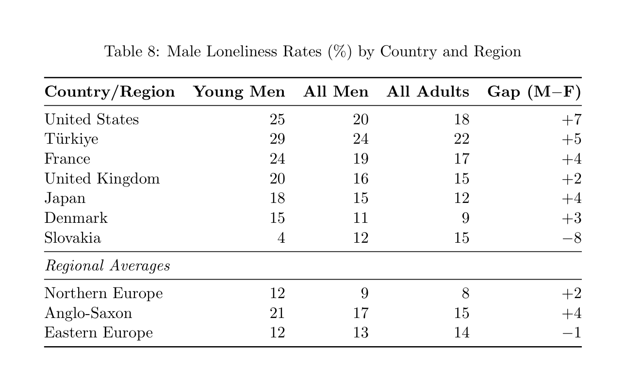
Table 8: Male Loneliness Rates (%) by Country and Region

Country/Region Young Men All Men All Adults Gap (M−F)

United States 25 20 18 +7 T¨urkiye 29 24 22 +5 France 24 19 17 +4 United Kingdom 20 16 15 +2 Japan 18 15 12 +4 Denmark 15 11 9 +3 Slovakia 4 12 15 −8

Regional Averages

Northern Europe 12 9 8 +2 Anglo-Saxon 21 17 15 +4 Eastern Europe 12 13 14 −1

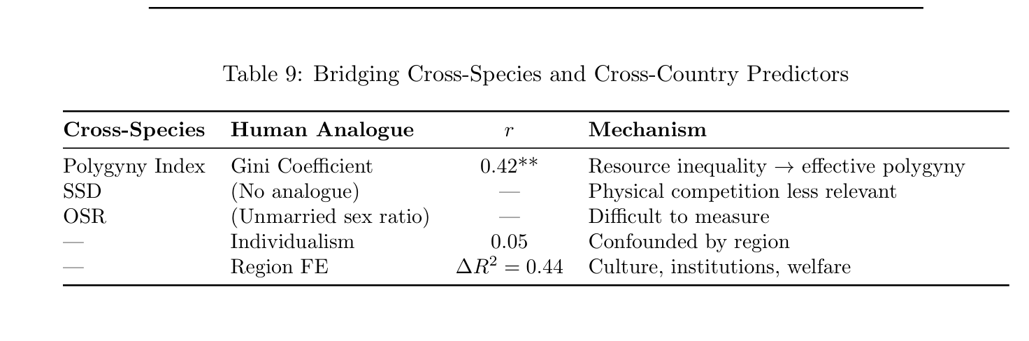
Table 9: Bridging Cross-Species and Cross-Country Predictors

Cross-Species Human Analogue r Mechanism

Polygyny Index Gini Coefficient 0.42** Resource inequality →effective polygyny SSD (No analogue) — Physical competition less relevant OSR (Unmarried sex ratio) — Difficult to measure — Individualism 0.05 Confounded by region — Region FE ∆R2 = 0.44 Culture, institutions, welfare

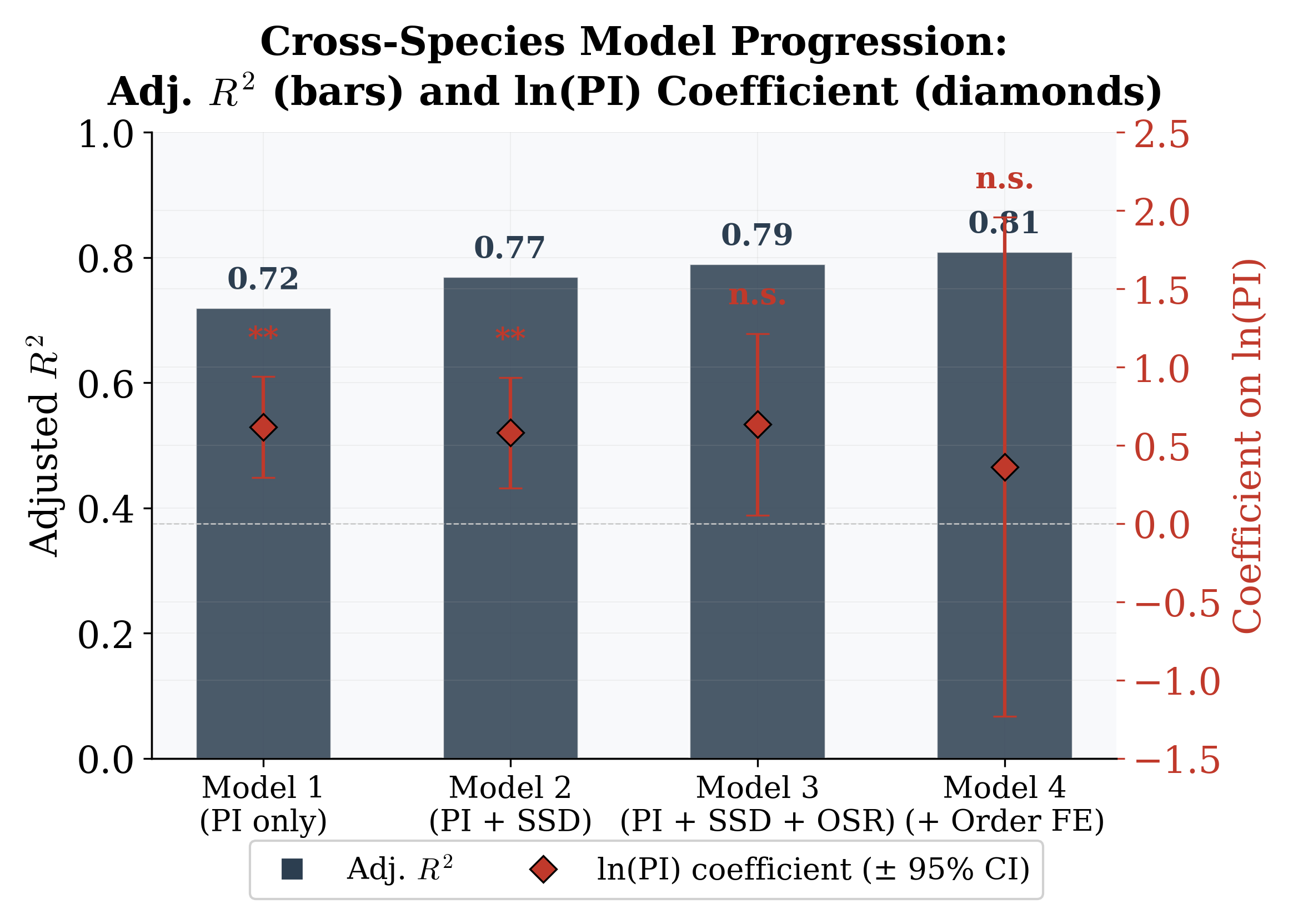
Figure 6: Cross-species model progression: Adjusted R2 (bars) and coefficient on ln(PI) with 95% CIs (diamonds). Adding SSD and OSR provides minimal improvement; order FE yield the largest incremental gain.

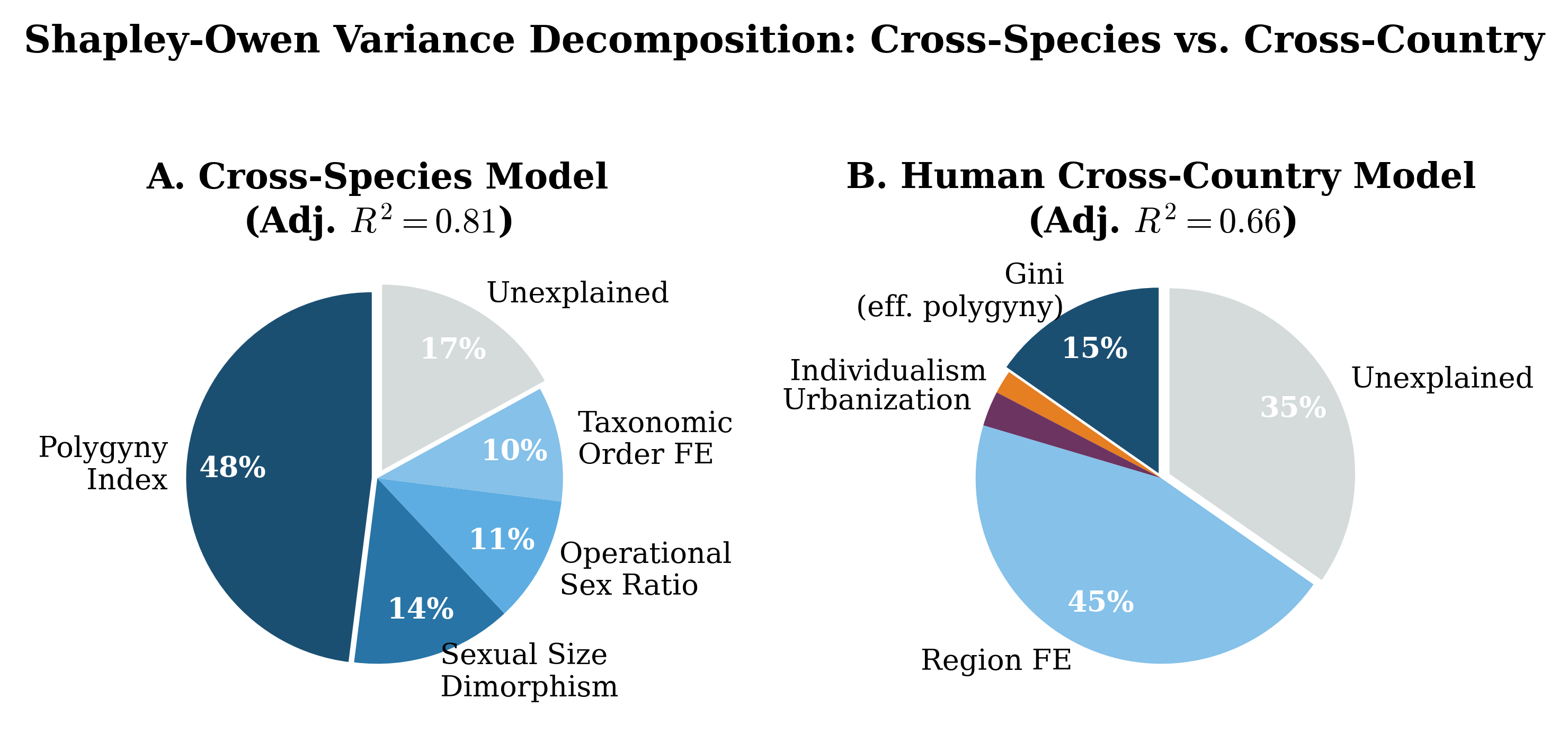
Figure 7: Shapley-Owen variance decomposition for the cross-species model (left) and cross- country model (right). The polygyny index dominates cross-species; region FE dominate cross-country.

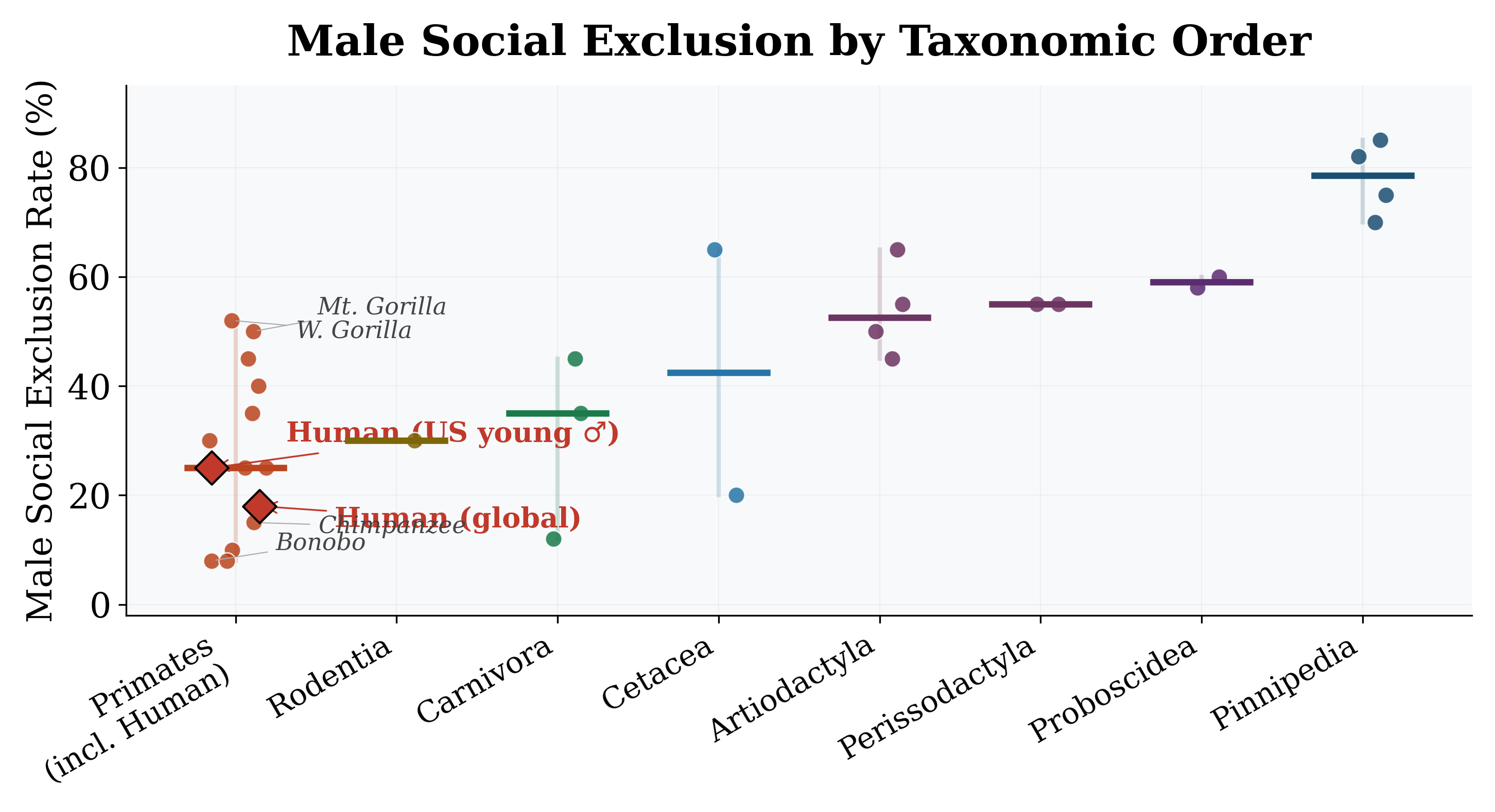
Figure 8: Distribution of MSER by taxonomic order. Pinnipeds show the highest median MSER; monogamous orders show the lowest.

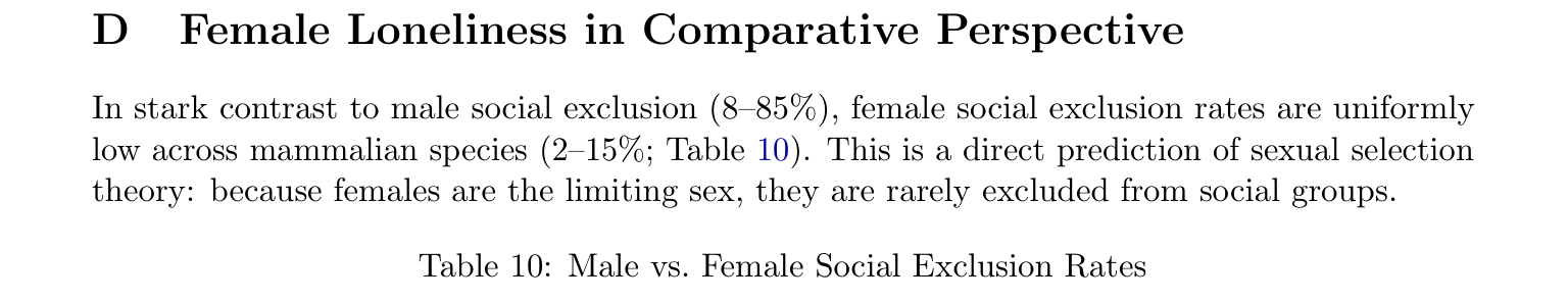
D Female Loneliness in Comparative Perspective

In stark contrast to male social exclusion (8–85%), female social exclusion rates are uniformly low across mammalian species (2–15%; Table 10). This is a direct prediction of sexual selection theory: because females are the limiting sex, they are rarely excluded from social groups.

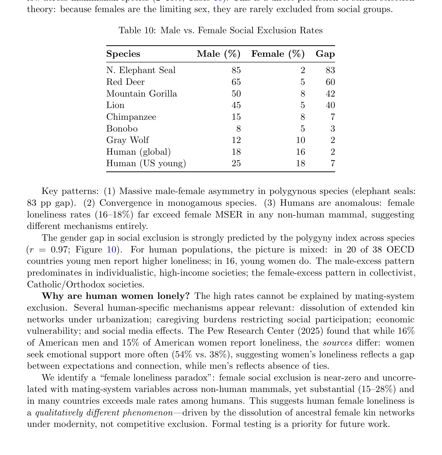
Table 10: Male vs. Female Social Exclusion Rates

Species Male (%) Female (%) Gap

N. Elephant Seal 85 2 83 Red Deer 65 5 60 Mountain Gorilla 50 8 42 Lion 45 5 40 Chimpanzee 15 8 7 Bonobo 8 5 3 Gray Wolf 12 10 2 Human (global) 18 16 2 Human (US young) 25 18 7

Key patterns: (1) Massive male-female asymmetry in polygynous species (elephant seals: 83 pp gap). (2) Convergence in monogamous species. (3) Humans are anomalous: female loneliness rates (16–18%) far exceed female MSER in any non-human mammal, suggesting different mechanisms entirely. The gender gap in social exclusion is strongly predicted by the polygyny index across species (r = 0.97; Figure 10). For human populations, the picture is mixed: in 20 of 38 OECD countries young men report higher loneliness; in 16, young women do. The male-excess pattern predominates in individualistic, high-income societies; the female-excess pattern in collectivist, Catholic/Orthodox societies. Why are human women lonely? The high rates cannot be explained by mating-system exclusion. Several human-specific mechanisms appear relevant: dissolution of extended kin networks under urbanization; caregiving burdens restricting social participation; economic vulnerability; and social media effects. The Pew Research Center (2025) found that while 16% of American men and 15% of American women report loneliness, the sources differ: women seek emotional support more often (54% vs. 38%), suggesting women’s loneliness reflects a gap between expectations and connection, while men’s reflects absence of ties. We identify a “female loneliness paradox”: female social exclusion is near-zero and uncorre- lated with mating-system variables across non-human mammals, yet substantial (15–28%) and in many countries exceeds male rates among humans. This suggests human female loneliness is a qualitatively different phenomenon—driven by the dissolution of ancestral female kin networks under modernity, not competitive exclusion. Formal testing is a priority for future work.

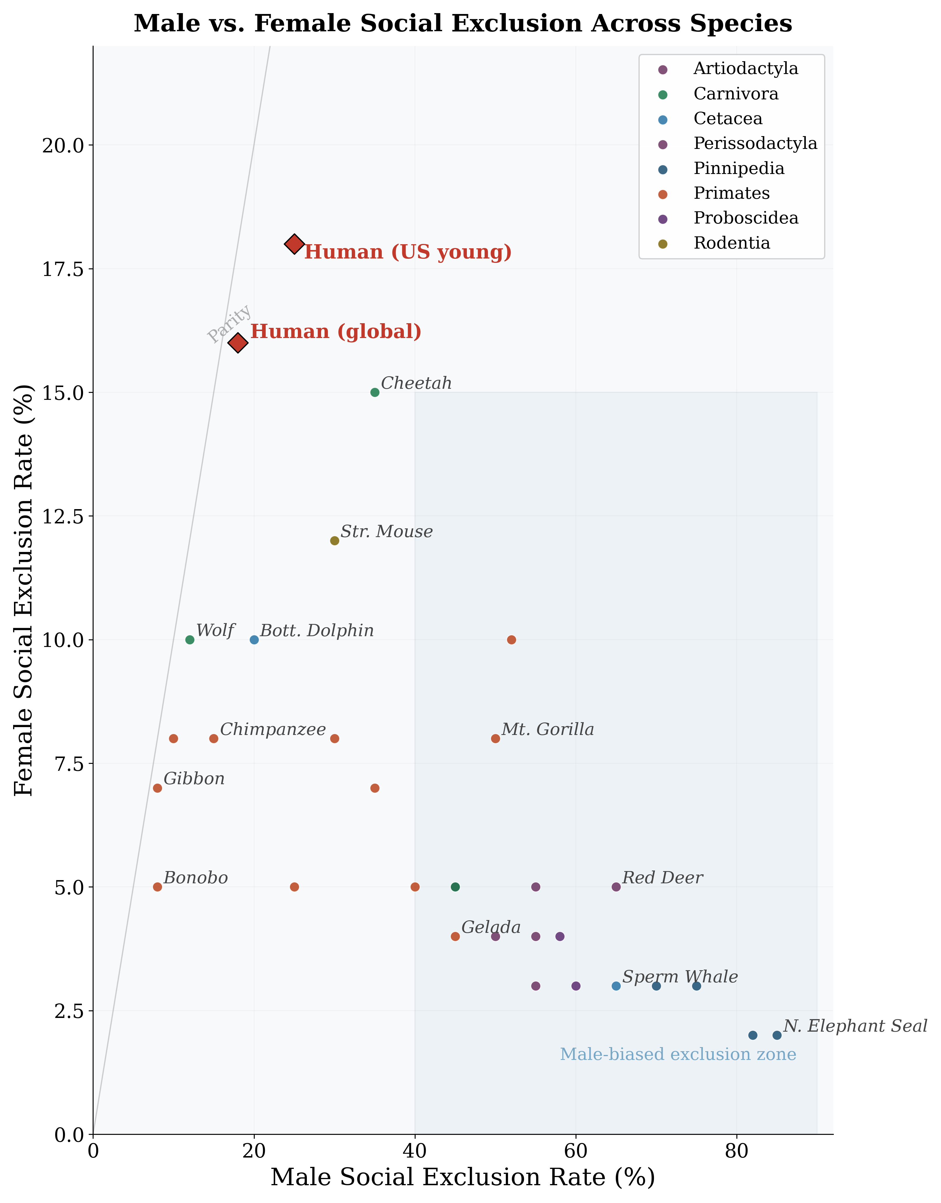
Figure 9: Male vs. female social exclusion rates across species. Highly polygynous species show massive asymmetry; humans cluster near the parity line.

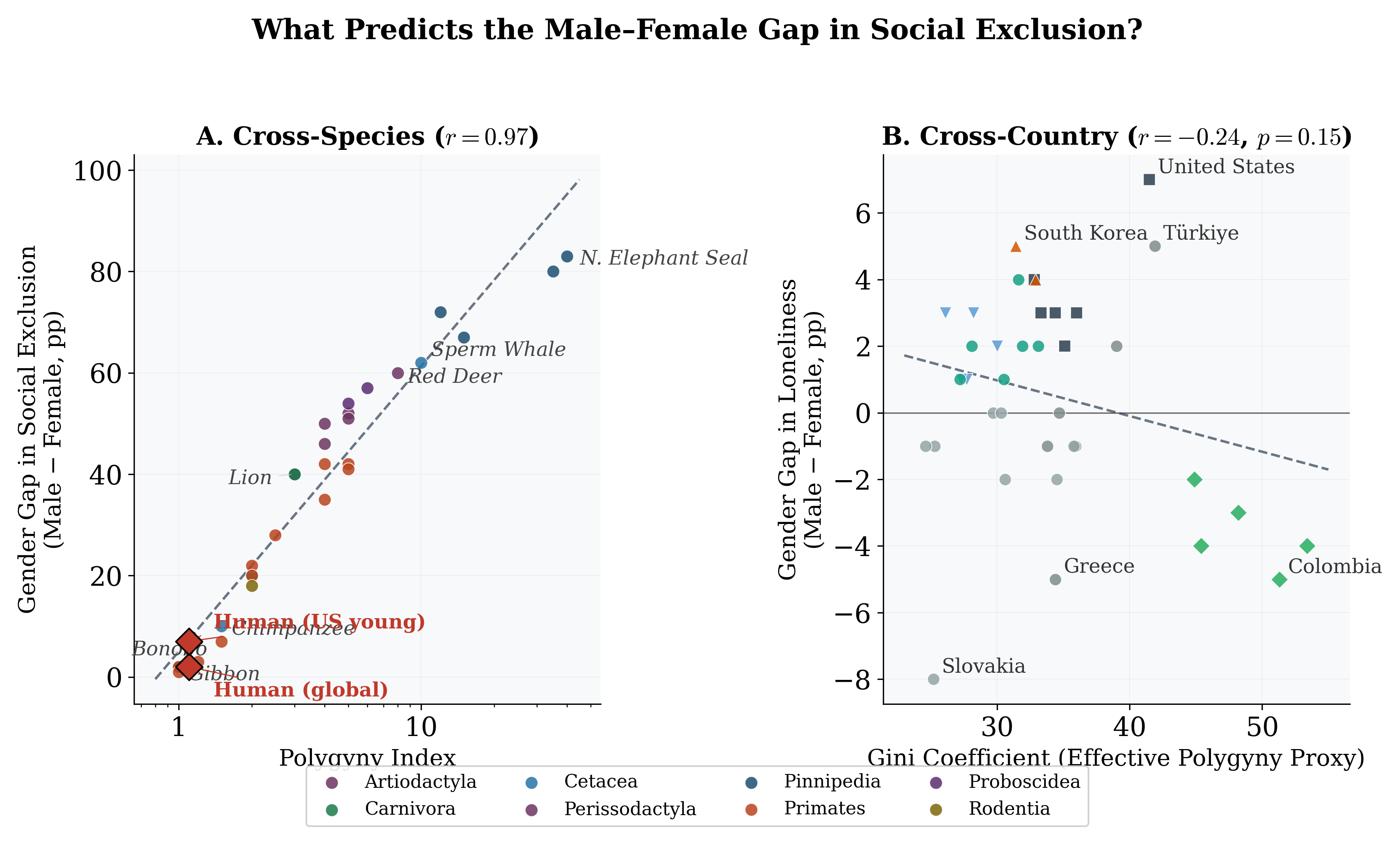
Figure 10: Gender gap in social exclusion as a function of the Polygyny Index (Panel A, cross- species, r = 0.97) and the Gini coefficient (Panel B, cross-country).

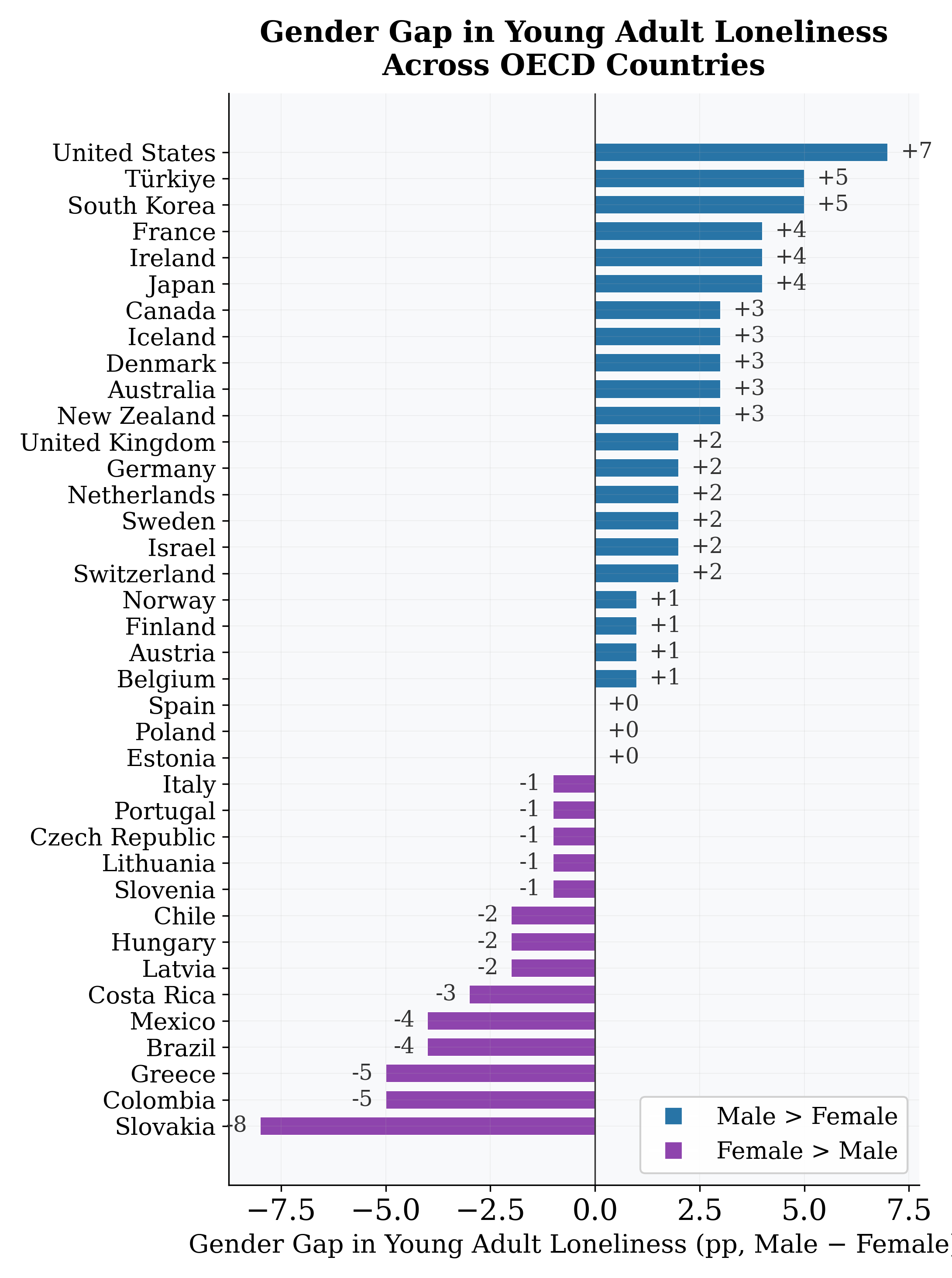
Figure 11: Gender gap in loneliness (male −female) across OECD countries.

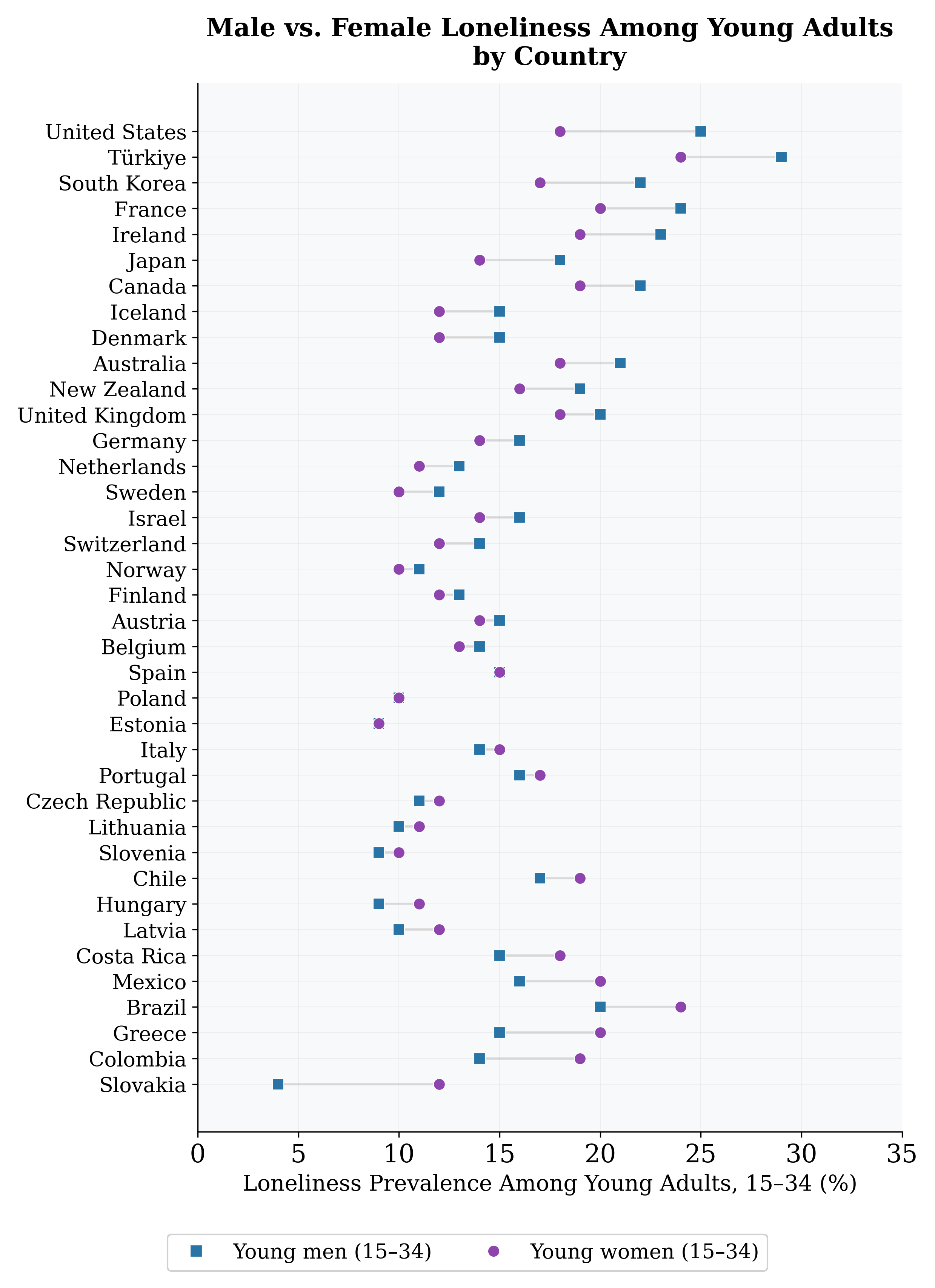
Figure 12: Male vs. female loneliness rates across countries. Points above the diagonal: male- excess loneliness.

E Robustness Checks and Limitations

E.1 Robustness Checks

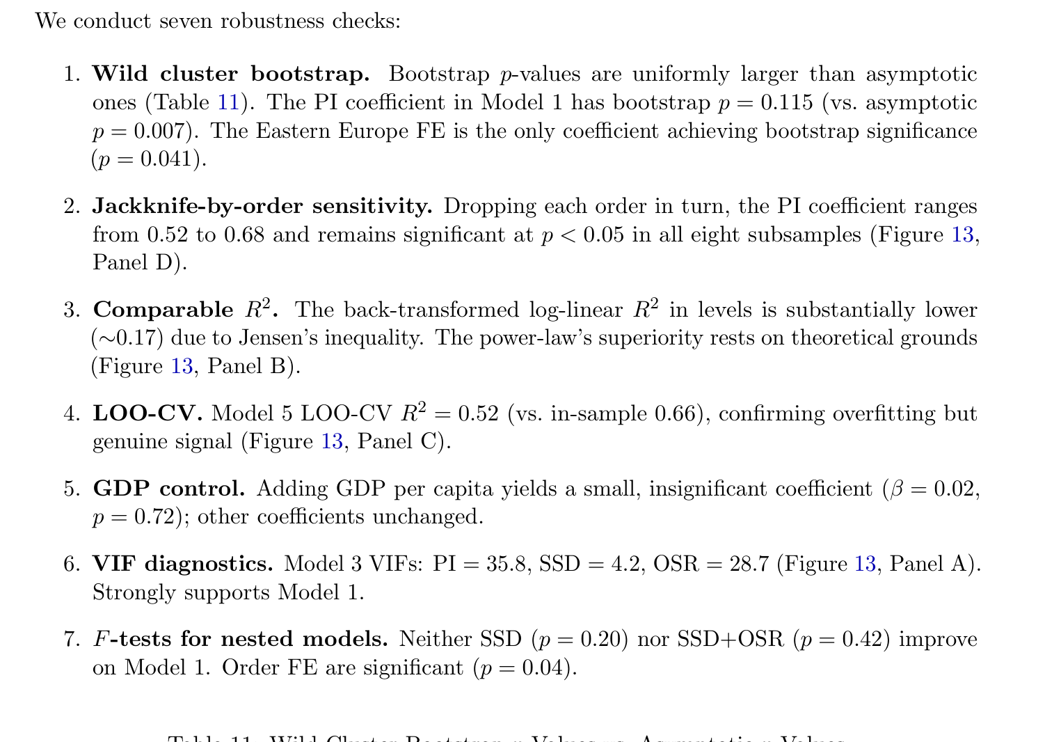
We conduct seven robustness checks:

1. Wild cluster bootstrap. Bootstrap p-values are uniformly larger than asymptotic ones (Table 11). The PI coefficient in Model 1 has bootstrap p = 0.115 (vs. asymptotic p = 0.007). The Eastern Europe FE is the only coefficient achieving bootstrap significance (p = 0.041).

2. Jackknife-by-order sensitivity. Dropping each order in turn, the PI coefficient ranges from 0.52 to 0.68 and remains significant at p < 0.05 in all eight subsamples (Figure 13, Panel D).

3. Comparable R2. The back-transformed log-linear R2 in levels is substantially lower (∼0.17) due to Jensen’s inequality. The power-law’s superiority rests on theoretical grounds (Figure 13, Panel B).

4. LOO-CV. Model 5 LOO-CV R2 = 0.52 (vs. in-sample 0.66), confirming overfitting but genuine signal (Figure 13, Panel C).

5. GDP control. Adding GDP per capita yields a small, insignificant coefficient (β = 0.02, p = 0.72); other coefficients unchanged.

6. VIF diagnostics. Model 3 VIFs: PI = 35.8, SSD = 4.2, OSR = 28.7 (Figure 13, Panel A). Strongly supports Model 1.

7. F-tests for nested models. Neither SSD (p = 0.20) nor SSD+OSR (p = 0.42) improve on Model 1. Order FE are significant (p = 0.04).

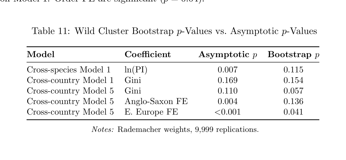
Table 11: Wild Cluster Bootstrap p-Values vs. Asymptotic p-Values

Model Coefficient Asymptotic p Bootstrap p

Cross-species Model 1 ln(PI) 0.007 0.115 Cross-country Model 1 Gini 0.169 0.154 Cross-country Model 5 Gini 0.110 0.057 Cross-country Model 5 Anglo-Saxon FE 0.004 0.136 Cross-country Model 5 E. Europe FE <0.001 0.041

Notes: Rademacher weights, 9,999 replications.

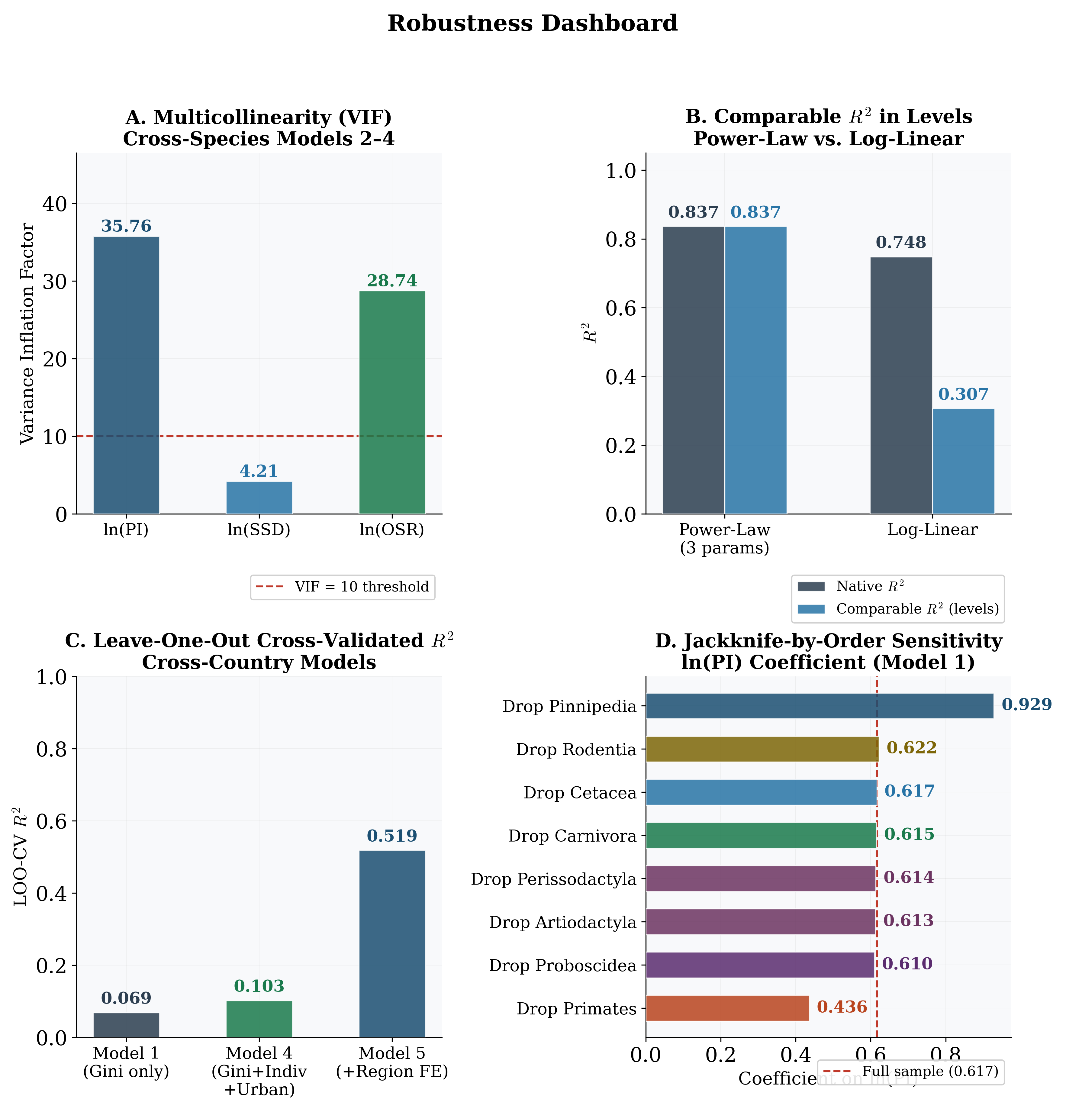
Figure 13: Robustness diagnostics. (A) VIFs for cross-species Models 2–3. (B) Comparable R2

in levels. (C) LOO-CV R2 for cross-country models. (D) Jackknife-by-order sensitivity.

E.2 Limitations

1. Construct validity. Non-human MSER and human loneliness are structurally analo- gous but phenomenologically distinct. Cross-domain comparisons should be interpreted cautiously.

2. Phylogenetic non-independence. Order-level FE are a crude correction; PGLS with a dated supertree (Felsenstein, 1985; Freckleton, Harvey, & Pagel, 2002) would be preferable. The jackknife provides partial reassurance.

3. Species sampling bias. The 29-species sample overrepresents large-bodied, well-studied species. Bats and insectivores are absent.

4. Bachelor group heterogeneity. Our MSER treats all males outside breeding groups as

“excluded,” but bachelor groups are often functional social units (Caro, 1994).

5. Endogeneity. Cross-country regressions are conditional correlations, not causal estimates. Instrumental variable or quasi-experimental designs are needed.

6. Overfitting. Adding 6 region dummies to 38 observations is aggressive; LOO-CV R2

(0.52) confirms genuine signal but substantial shrinkage.

7. Gender of loneliness. The “male loneliness epidemic” is concentrated in young men in high-income countries—not a universal pattern.

8. Female MSER estimates. Less well-documented than male rates; precise values carry uncertainty.