Holographic Fiber Theory (HFT) models the vacuum as an informationally discrete cell complex governed by a weaving rule: a combinatorial law for how cell states couple and update. Its first part is a trivalent connectivity whose continuum limit realises the Hopf bundle S³ → S². Its four cohomology channels pair by Poincaré duality into the substrate's two fields, a tension field and a phase field, and its homotopy classes supply the topological matter charges. Its second part is a braiding constraint on this connectivity, two-strand on each edge and three-strand at each vertex; a symmetry-breaking event locks the edge braid's chirality, fixing the gauge structure and prestressing the vacuum. Coarse-grained across cells and ordered by causal dependence, its deterministic updates read statistically as a signed-measure Markov chain, reproducing the Tsirelson bound from local, real-valued weights and delivering the path-integral measure; the same operator's short-time heat kernel returns the form of the Einstein–Hilbert curvature term, and the Lorentzian metric is stitched in the infrared by a signal speed binding tick count to spatial span. The coarse-graining mechanism is checked by accompanying scripts rather than posited. The Standard-Model mass spectrum emerges as energy topologically trapped in the prestressed tension field. Two near-term falsifiable targets from the tension floor: the summed Majorana neutrino mass, Σm_ν ≈ 61.2 meV, and the cosmic neutrino background temperature T_CνB = T_CMB ≈ 2.725 K, the two backgrounds sharing one thermal fluctuation — an irreducible entropic cost rather than a frozen relic, read in the finite-information frame this paper adopts.
1 Introduction
The hard part of a discrete substrate is the coarse-graining: what carries it to continuous field theory, and whether that can be made explicit. Holographic Fiber Theory (HFT) carries it by the weaving rule itself, drawn as an explicit geometric construction in three dimensions and executable as a machine — a coarse-graining that can be computed and run. What the same rule supplies differs at each level of description: the wiring at the bottom, the measure over histories in the middle, the field equations at the top.
Its cells are discrete in information rather than in coordinates: by the holographic principle [1, 2] the information in a region is bounded by its area, so each cell holds finitely many states while position and direction stay continuous. The rule's first part is a trivalent connectivity realising the Hopf bundle [3] \( S^3 \xrightarrow{S^1} S^2 \), whose channels pair into the two fields the substrate carries, a cell tension \( \rho \) and a Hopf-fiber phase \( \psi \); its second is a braiding on that connectivity, doubled along each edge and three-fold at each vertex, whose handedness one locking event fixes — installing the non-abelian gauge groups and prestressing the vacuum (§3).
The substrate evolves in discrete ticks, each costing one action quantum \( \bar{h} \), and time is the coarse-grained rise of entropy along that sequence. Closing a cyclic update carries an irreducible entropy cost, which keeps the theory ultraviolet-finite without a renormalisation cutoff.
Together these fix what a coarse-graining can read off the substrate: the quantitative results that follow from counting cell states, the Einstein field equations from the elastic response of the tension field, and quantum field theory from two successive coarse-grainings of that counting.
2 Methodological Preliminaries
| Structural commitment | What it is, and what it supplies |
|---|---|
| Cell complex | Finite-state cells coarse-graining to two fields \( \rho, \psi \), supplying the information slots: coupling ratios, UV finiteness, and emergent time. |
| Hopf bundle | The bundle \( S^3 \xrightarrow{S^1} S^2 \) (\( S^2 \) field base, \( S^1 \) phase fiber), supplying connectivity: the cohomology channels \( H^0 \)–\( H^3 \) and the \( \pi_n \) solitons (charge, isospin, baryon #). |
| Braiding | \( B_2 \) on edges and \( B_3 \) at vertices, constraining how strands cross that connectivity and supplying the gauge sector: \( SU(2)_L \), \( SU(3)_C \), and the chirality lock that reproduces CP breaking. |
(1) Unit-free weaving rule. The weaving rule carries no intrinsic length scale and no specific microscopic form: it fixes only how cell states couple and transition. Every derived constant is thus a dimensionless count or ratio, the Planck mass \( m_P \) entering only as the ruler that sets SI units, so the weaving rule is also parameter-free. The rule therefore stands for the whole class of local, asynchronous, ledger-conserving updates. Every infrared result is then a class invariant, fixed like a critical exponent by symmetry and conservation rather than by a microscopic Hamiltonian; the class's state schema, axioms, and update interface delimit the theory's scope, and one explicit realisation is written out as a witness rather than a further commitment (App. H). The rule is the coarse-graining itself rather than any level of description (§9).
(2) Holographic-discrete, not lattice-discrete. The substrate's discreteness is in information, not in coordinates — an it-from-bit ontology [4] carried down to the cell. By the holographic bound each cell holds finitely many distinguishable states, so what is discrete is the microstate content the slot count tallies; the Planck-scale cell (App. G) is then a resolution threshold, not a quantum of position. Position and direction stay continuous, determined relationally at each interaction rather than stored on a grid — the substrate a continuum of finite information density, not a lattice of quantised coordinates.
(3) Geometry and field theory are coarse-grained readouts. Every geometric and field-theoretic term in this paper — surfaces, angles, phases, and fiber bundles, and equally the continuum time, action, path integral, and Hilbert space — is a coarse-grained readout of that state-counting, an aid for reading the weaving rule rather than a fundamental entity. An "angle" is a discrete capacity fraction, and a "2π phase" a completed cyclic orbit of a cell's finite state space.
3 The Geometric Framework
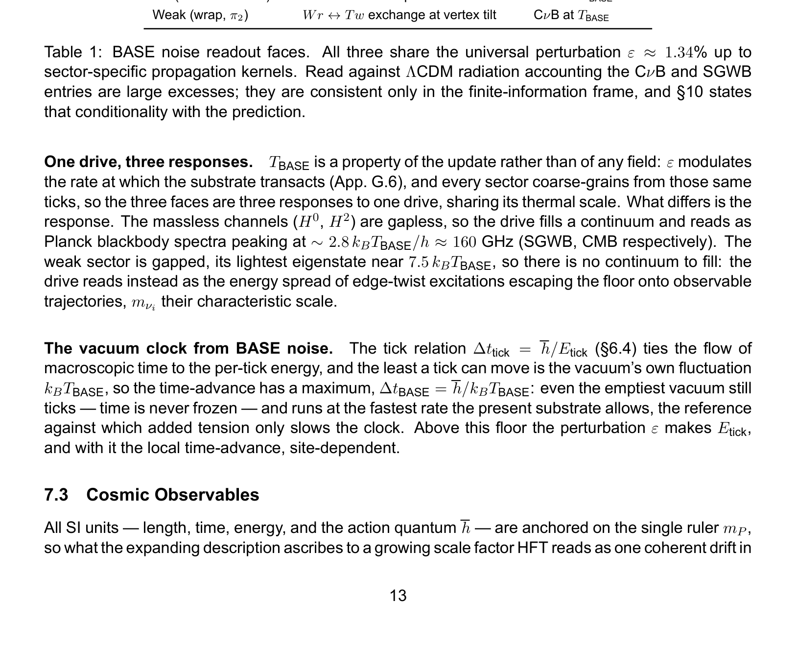
Figure 1: A connectivity dual, not a lattice. The figure depicts only the combinatorial adjacency of the cell complex (black, triangular) and its trivalent honeycomb dual (blue) with one vertex at each cell's centroid and \( N_v = 3 \) edges to the three sides.
3.1 Connectivity, Distance, and the Bundle
Every geometric term below — surface, direction, angle, bundle — is a coarse-grained readout of finite state-counting, as §2(3) commits and §9 works out; a reader unwilling to grant that may go there first. On that footing the geometry is used freely.
Connectivity. The connectivity is trivalent: each cell carries one vertex and \( N_v = 3 \) edges, and nothing further about its shape is fixed. Each edge is a half-edge in the combinatorial-map sense, belonging to one cell alone, and two edges joined across adjacent cells form a bond (Fig. 1). The triangles of the figure are only how such a complex is drawn, and the degree is derived rather than chosen (App. I).
Distance as a count of relations. No cell stores a coordinate, so a separation is a count rather than a container: how many update relations stand between two cells, the order and the count both supplied by the axioms of App. H. Both of the substrate's spatial structures are relations of that kind — the trivalent adjacency across the base, and the fiber phase mismatch between two cells, which neither cell stores — and both are counted in one unit: a single update relation, which reads out at the Planck scale (§2(2)).
Emergent isotropy. Every spatial direction the coarse-graining returns is such a count in that same unit, so the emergent metric has nothing by which to tell one from another (App. F). No cell stores an axis; the three spatial directions are fixed relationally at each interaction, an axis being a relational readout rather than a stored quantity. Whatever asymmetry there is in how the substrate encodes a direction is therefore a distinction among its degrees of freedom, not among the directions themselves.
The bundle's contribution. The Hopf bundle \( S^3 \xrightarrow{S^1} S^2 \) (Euler class 1) fixes how many independent readouts a cell has, two across the \( S^2 \) base and one along the \( S^1 \) fiber; it sorts the modes into the four cohomology channels (§3.3); and it carries the topological charges (§4.2). Depth is common to all three directions; what is particular to the fiber is charge.
3.2 Chirality lock: a brief geometric picture
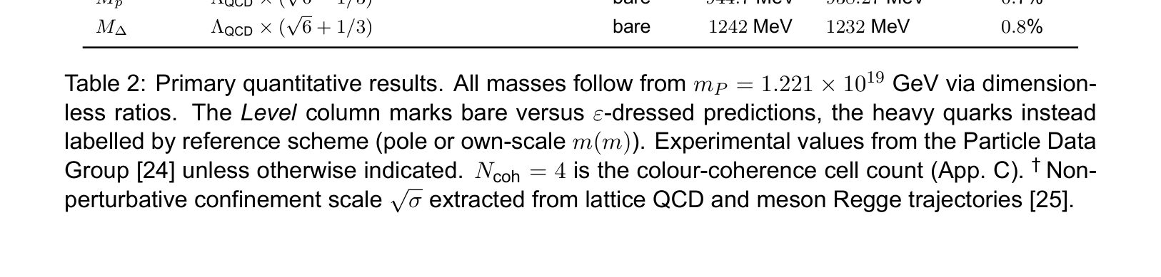
Figure 2: Visualisation of the weaving rule at a locked vertex and its edges, viewed inward, down the axial \( S^1 \) fiber (black dot); the strands are not physical primitives, only a depiction of its topological constraints on the connectivity.
Strands at edges and vertices. Each edge carries a two-strand framed thread (braid group \( B_2 \)) with a \( \mathbb{Z}_2 \) handedness label; each vertex is a single \( S^1 \) axial fiber threaded by three strands, \( C_3 \)-symmetric (120°) about that axis, each linking a different pair of the vertex's incident edges — so every edge carries two. The vertex braidings realise \( B_3 \), a trivial vertex sitting at the unbraided identity.
The lock. A single global event breaks the substrate's parity symmetry: each edge becomes a left-handed \( B_2 \) braid, each vertex a left-handed \( B_3 \) trefoil (Fig. 2). That the lock occurs is derived rather than posited; which handedness it installs is not (App. I).
Post-lock stress substrate. Post-lock, the two strands of each edge differentiate into an axial anchor strand, pulled taut, and a helical free-carrier wound around it. Their roles are positional, not fixed to a strand: at each vertex the anchor turns out as the carrier of the next bond and the carrier as the next anchor, under the one handedness the lock fixed, so a strand regains its own role only after two vertices. This double cover of its role worldline is a \( \mathbb{Z}_2 \) structure that recurs as a structural pillar of the emergent field theory (§9).
The three twist modalities. The free-carrier strand's residual twist freedom organises into exactly three modalities, one at each of three nested levels: the strand's self-twist (\( Tw_{sub} \)), the carrier's wrap around the anchor (\( Tw_{wrap} \)), and the collective twist of the whole edge as a single Hopf fiber (\( Tw_{Hopf} \)).
Topological solitons. The Hopf bundle carries one topological soliton per homotopy degree \( \pi_n \): a vortex (\( \pi_1 \)), a \( \psi \)-phase defect with a core; a skyrmion (\( \pi_2 \)), the strand wound around the axial fiber; and a hopfion (\( \pi_3 \)), a knotted cage of \( \rho \)-tension. These three are the topological primitives from which the Standard-Model particles and their charges are built (§4.2).
Twist and writhe. A twist and a writhe are two forms of one linking, exchanged at fixed \( Lk = Tw + Wr \) by the Călugăreanu identity [5, 6, 7]. So the free carrier's wrap about the anchor on the edge, \( Tw_{wrap} \), pairs to a \( Wr_{wrap} \) at the vertex — a wrap about the axial fiber (Fig. 2); the collective twist \( Tw_{Hopf} \) pairs to a knotted vertex \( Wr_{Hopf} \). The strands depict constraints on the connectivity, not primitives, so topologically we may picture \( Wr_{wrap} \) as a writhe on \( S^2 \), a skyrmion, and \( Wr_{Hopf} \) as a writhe on \( S^3 \), a hopfion.
3.3 Cohomology Channels
The substrate's topology partitions its modes by form degree: four channels, written \( H^0 \)–\( H^3 \) after the degree each occupies, one for each degree of the 3D substrate — the Hopf bundle's \( S^1 \) fiber and \( S^2 \) base supplying the middle two: a scalar tension (\( H^0 \)), the fiber connection one-form (\( H^1 \)), the base flux two-form (\( H^2 \)), and the top volume form (\( H^3 \)). Each carries a distinct topological mode type into which the elastic energy localises, giving one IR field:
| Class | Substrate content | IR field |
|---|---|---|
| \( H^0 \) | long-wavelength tension across the cell complex | gravitational field (§6) |
| \( H^1 \) | phase holonomy across the \( S^1 \) fiber | gauge potential \( A \) (charge) |
| \( H^2 \) | Euler-class flux across the \( S^2 \) base | photon field strength \( F \) |
| \( H^3 \) | inter-fiber braid at the vertex | gluon field (colour) |
The four channels are two fields — the tension \( \rho \) and the phase \( \psi \) — each read through a Poincaré-dual pair of degrees on the closed oriented 3-substrate (the Hopf total space \( S^3 \)): \( \rho = (H^0, H^3) \), a metric-free global pair, and \( \psi = (H^1, H^2) \), the metric-dependent local Hopf fiber–base pair.
The same two-field division reappears in the infrared as the symmetric and antisymmetric halves of the rank-two frame edge:
$$ \text{edge} \otimes \text{edge} = \underbrace{\text{Sym}^2(\text{edge})}_{\text{metric } (\rho)} \oplus \underbrace{\Lambda^2(\text{edge})}_{\text{field strength } (\psi)}. \tag{1} $$
The traceful symmetric half stretches the two edge directions together, a change of volume and tension, and reads out as the metric (gravity, the \( \rho \) pair). The traceless antisymmetric half pushes one against the other, a local rotation of the frame, and reads out as the field strength (the photon, the \( \psi \) pair). This traceful–traceless split is what later distinguishes the gravitational \( 8\pi \) coupling from the bare \( 4\pi \) of a field strength. The Lorentz indices these fields carry are themselves emergent: eigenmode labels of the substrate's discrete Laplacian (App. F.2).
The cell's continuum phase space. Read in the continuum, a cell carries
$$ \mathcal{Q} = \mathbb{R}^+ \times S^2 \times S^1_{Hopf}, \tag{2} $$
-
\( \mathbb{R}^+ \) (1 DOF): the cell tension \( \rho \) — its information load, how much of its finite capacity is in use — read macroscopically as energy. Its IR coarse-graining is the substrate's classical tension field, whose local value an observer measures as mass-energy density.
-
\( S^2 \) (2 DOF): the two base directions, read from the connectivity, supplying two of the three coordinates of relational position.
-
\( S^1_{Hopf} \) (1 DOF): the fiber phase \( \psi \), whose mismatch between cells supplies the third coordinate, depth. The identification is operational, made afresh at each interaction: phase-resonant configurations interact strongly and read as adjacent, while phase-orthogonal ones cannot interact and read as depth-separated, so the information-theoretic phase mismatch is the geometric depth.
Only the field values are stored: \( \rho \) and \( \psi \) are what a cell encodes, and §3.4 tallies them; the base directions are relational, held by no cell (§3.1).
3.4 The Cell's Core Slot Count
The phase space fixes what each cell encodes: beyond its position, the two field values, the tension \( \rho \) and the phase \( \psi \) — collective variables whose smooth forms \( \rho(x), \psi(x) \) emerge only in the many-cell average (App. F.2). The Hopf bundle and its braiding fix how many states the cell carries and how they flow through its cohomology channels. We trace the phase field \( \psi \) — the photon's — through one cell, element by element.
Encoding dynamics. The substrate advances in discrete ticks, each cell rewriting its finitely many states one tick at a time (§6.4); a field's microscopic dynamics is therefore the change from one tick to the next, not anything held within a single tick. Each primitive carries one bit per tick, and pairing two ticks — (now, next) — shows whether the value flows. Held (now = next) it reads static, a standing value; changing (now ≠ next) it reads dynamic, a value in flow. A direction takes two ticks to define and so is not a stored value either; spin follows from the history (App. D.3).
Reading an edge. On a single strand, \( \psi \)'s held part (now = next) is a standing field value — the static Coulomb flux a charge at rest maintains through the base; its changing part (now ≠ next) is the phase advancing with a definite sense — what the many-cell readout assembles into a mode propagating across the field. An edge carries two such strands (\( B_2 \)), so it holds \( 2 \times \) (now, next): four bits, \( 2^4 = 16 \) slots. On the edge \( \psi \) is the base channel \( H^2 \), the photon field strength \( F \).
Reading the vertex. At the vertex \( \psi \) has two further primitives — the \( S^1 \) axial fiber threading it, and the cross-point where the three edges meet in the base — four more bits, sixteen more slots, two samples of the one fiber potential. On the axial fiber its holonomy is the charge: a steady value (now = next) reads as the standing potential \( A_0 \) of a charge at rest, a changing one (now ≠ next) as a current along the fiber. At the cross-point a steady value reads as the standing phase at which the three edges meet, a changing one as that junction phase advancing. Here \( \psi \) is the fiber channel \( H^1 \), the gauge potential \( A \) — the phase holonomy along the fiber; its field strength \( F \) (\( H^2 \)) is the curvature read on the edges, not a second quantity stored at the vertex.
Counting the slots. Across its four elements — three edges and the vertex — the phase field occupies \( (3 + 1) \times 16 = 64 \) slots, \( N_\psi = 64 \). The tension field \( \rho \) fills a second 64 by the same count, \( N_\rho = 64 \), and the two fields add:
$$ N_\rho + N_\psi = 128. \tag{3} $$
4 The Standard Model from the Locked Mesh
The chirality lock reshapes the substrate: it activates the braid-reconnection gauge groups, grows a strong-sector block of new slots, and fixes the topological charges that label matter.
4.1 Gauge groups as conversion operators
The non-abelian gauge groups are not channels but conversion operators acting on \( \rho \) and \( \psi \): continuous algebras of braid reconnection at each site, \( SU(2)_L \) on the edge \( B_2 \) and \( SU(3)_C \) on the vertex \( B_3 \), the way the chirality lock reaches into the two fields and converts their content. They carry no field of their own: a \( W \), \( Z \), or gluon is read out only through the mass (\( \rho \)) and charge (\( \psi \)) it disturbs, so what the IR continuum renders as a Yang–Mills field is the propagating disturbance these operators leave in the two fields.
Electroweak: \( SU(2)_L \times U(1)_Y \). The abelian factor is the phase of the \( S^1 \) Hopf fiber, and its holonomy is the electric charge \( Q \). Before the chirality lock this factor is the hypercharge \( U(1)_Y \); once the lock has acted the physical fiber holonomy is \( Q \).
Before the lock the edge's two strands, an anchor and a carrier, are interchangeable. The chirality lock picks the anchor: the trace settles on that taut anchor strand, the gravitational tension \( H^0 \), while the traceless \( su(2) \) acts on the left-handed states alone — \( SU(2)_L \), a conversion operator on the edge \( B_2 \). Its diagonal generator is the weak isospin \( T_3 \) and its off-diagonal generators the charge-changing \( W^\pm \). This conversion crosses the lock's misalignment between the \( \rho \) strand content and the \( \psi \) fiber, whose size is the Weinberg angle \( \theta_W \) (§5.3) mixing \( U(1)_Y \) with \( SU(2)_L \); the surviving abelian charge is the physical electric charge \( Q \), the net fiber holonomy.
Strong: \( SU(3)_C \). The three strands meeting at each vertex carry the three colours, and post-lock they braid around the vertex — the \( B_3 \) braid. Its crossings do not commute, and this non-commuting content is the \( su(3) \) of eight gluons: a gluon is a crossing that passes one strand over another, swapping their colour labels. The braid's abelian part — the net winding shared by all three strands — commutes with every crossing and is conserved as baryon number, the trace \( u(1)_B \). The three-strand rotation thus spans the full \( u(3) \): eight gluons and one baryon-number charge.
4.2 The particle spectrum
Every matter particle is a localised packet of \( \rho \)-stress on the chirality-locked mesh, held against dispersal by the topological charges its region carries; that trapped stress is its mass. This section lays out the spectrum qualitatively; the quantitative mass derivations follow in App. B–C.
The topological quantum numbers. The substrate's charges are the Hopf bundle's topological solitons, one per homotopy degree \( \pi_n \), each a signed winding read looking inward along the axial fiber, clockwise counted \( + \), counter-clockwise \( - \), in the standard \( R = +, L = - \) assignment, so reversing the winding sends a particle to its antiparticle. The vortex pairs the \( \psi \)-phase with its curvature, the Coulomb flux; the skyrmion and hopfion join an edge twist to its vertex writhe by the Călugăreanu identity \( Lk = Tw + Wr \). They are
| Object | \( \pi_n \) | Topologically conserved | SM readout |
|---|---|---|---|
| vortex | \( \pi_1(S^1) \) | Yes — stable in 3D | electric charge \( Q \) |
| skyrmion | \( \pi_2(S^2) \) | No — unwinds in 3D | weak isospin \( T_3 \) (left-handed) |
| hopfion | \( \pi_3(S^2) \) | Yes — stable in 3D | baryon number \( B \) |
Charge. Electric charge — the vortex (\( \pi_1 \)) above — is the winding of the \( S^1 \) fiber phase, the \( H^1 \) holonomy, and it wears two faces the Hopf bundle ties together: along the fiber it is the gauge potential \( A \) (\( H^1 \)), and around the carrier in the base it is the Euler-class flux \( F \) (\( H^2 \)), the Coulomb field.
Weak isospin. The skyrmion (\( \pi_2 \)) is the wrap — a carrier strand wound once about the anchor, carried on the vertex writhe \( Wr_{wrap} \) with the edge twist \( Tw_{wrap} \) its edge form. Being the left-handed braid the lock installed, the wrap sits only on left-handed states (the right-handed ones are wrap-free \( SU(2) \) singlets) and carries the one fixed handedness, so weak isospin \( T_3 \) reads its presence, not its sign: the down-type wrapped, the up-type not. The \( SU(2)_L \) conversion (§4.1) adds or removes a wrap, moving it between the edge twist and the vertex writhe; its charged form \( W^\pm \) is what turns a down-type into an up-type. Carrying no winding the topology protects, the skyrmion is unstable in three dimensions — which is why weak isospin alone is not conserved.
Charged leptons. A charged lepton is the simplest particle: a colourless vortex carrying the \( -1 \) charge, with no braid and no \( Wr_{Hopf} \) knot (\( B = 0 \)). Its generation is the number of wraps the carrier makes about that vortex — none for the electron, one for the muon, two for the tau — each adding trapped \( \rho \)-stress, so the mass climbs with the wrap count while the charge stays one unit. The electron, the bare vortex, is wrap-free and knot-free, hence the lightest, stable, and point-like. The triad's masses trace a single winding cone whose phase-independent participation ratio is the empirical Koide relation \( Q_{Koide} = 2/3 \) [8] (App. B).
Neutrinos. The three neutrinos are distinguished not by a \( Tw_{sub} \) count but by modality — which of the carrier's three sub-integer edge twists (\( Tw_{sub} \), \( Tw_{wrap} \), \( Tw_{Hopf} \)) is perturbatively excited (§3.2). Sharing the one carrier, they mix freely. Carrying no integer winding, each has nothing to reverse and so is its own antiparticle; the locked edge's single handedness leaves no \( \nu_R \), so the mass can only be Majorana.
Hadrons: local and non-local colour closure. A baryon closes colour locally: three strands, the three colours, braid into a knot at one vertex, the \( SU(3)_C \) grip pinning a unit of \( Wr_{Hopf} \), the baryon number (App. E). The knot is an integer class no deformation undoes, so the lightest, the proton, is stable, its mass set by the confinement scale \( \Lambda_{QCD} \). A meson closes colour non-locally: a quark bridges to an antiquark at another vertex through a colour flux tube, a strand of \( \rho \)-stress running from a colour to its conjugate. The tube costs confinement energy, most of the meson's mass, but ties no knot (\( B = 0 \)). A tube can also close on itself, with no endpoints and no quark strands to carry flavour: the glueball, likewise unknotted.
Quarks. A quark is one strand's structure inside a hadron — its colour, its self-twist, its \( \pm 1/3 \) or \( \pm 2/3 \) share of the fiber winding. The fractional shares follow from closure (App. E): colour quantises a strand's winding in thirds, the weak wrap separates up-type from down-type by one unit, and fixing the proton \( uud = +1 \) and neutron \( udd = 0 \) forces \( u = +2/3, d = -1/3 \) — the integer hadron charge primary, the fractions its distribution across the strands. Yet no quark has a free state: the \( \rho \)–\( \psi \) substance holds no isolated strand, only the colour-closed hadron. Confinement is thus a structural identity, not a dynamical trap.
Gauge bosons. Unlike these trapped matter packets, a gauge boson is not a stored charge but the propagating disturbance a conversion operator (§4.1) leaves in the two fields. Whether it carries mass is a two-field question: a conversion that stays within one field is massless, while one bridging \( \rho \) and \( \psi \) pays the crossing as mass — so the gluon (within \( \rho \)) and the photon (within \( \psi \)) stay massless, and only the field-bridging electroweak sector gives the massive \( W \) and \( Z \).
Decay. A packet above its lowest energy state decays for either of two reasons. It may carry no conserved charge to pin it against reconnection — a stacked wrap or self-twist, or a knot that is not the lightest — so nothing resists its unwinding into neutrinos or radiation. The unknotted tubes are the plainest case: the meson and the glueball are legal, propagating, but transient concentrations, decaying as the tube breaks or, for the meson, as the pair annihilates. Or the packet's cells may saturate, expelling the surplus as energy once loaded to capacity, an exclusion kin to degeneracy pressure that leaves the most overloaded states the shortest-lived. A particle is stable only where both close off: the lightest carrier of a conserved charge — the electron (electric charge \( Q \)), the proton (baryon number \( B \)).
5 Coupling Constants from Substrate Slots
By coupling the strands at each vertex and edge, the lock turns the slot counts into measurable couplings: the friction it induces is the coupling each channel carries. The inventory below fixes those counts; each constant is then a ratio of those integers, read at its proper scale. Only that leading term is given here; the perturbative correction that separates it from measurement is taken up in App. A.
5.1 The Slot Inventory
§3.4 counted the electroweak–gravity core, \( \text{SLOT}_{EWG} = N_\rho + N_\psi = 128 \). This section completes the inventory the couplings below are ratios of.
The strong block. The lock braids the three colour strands at each vertex into \( B_3 \), making their pairwise tension-routing a new degree of freedom in \( \rho \): an \( N_v \times N_v \) matrix of strand-pair slots. Three are diagonal — each strand's own tension, held static — and six off-diagonal, the dynamic reconnections that route tension from one strand to another, so
$$ \text{SLOT}_{strong} = 3 + 6 = N_v^2 = 9, \qquad \text{SLOT}_{total} = \text{SLOT}_{EWG} + \text{SLOT}_{strong} = 137. \tag{4} $$
Coarse-grained, these same nine span the gauge algebra \( u(3) \): the six off-diagonal reconnections are the colour-changing gluons, the three diagonal recombining into the conserved baryon number (their symmetric sum) and two further gluons (the traceless remainder) — the eight-gluon octet and the baryon charge.
The edge carrier. One edge's \( \rho \) block holds sixteen slots: its two strands, anchor and free-carrier, each carry a (now, next) bit pair reading silent \( (0, 0) \), changing \( (0, 1)/(1, 0) \), or held \( (1, 1) \). Sorting the sixteen under the priority anchor-motion > held > carrier-motion:
| anchor \ carrier | silent (00) | changing (01),(10) | held (11) |
|---|---|---|---|
| silent (00) | vacuum ×1 | \( Tw_{sub} \times 2 \) | \( Tw_{wrap} \times 1 \) |
| changing (01),(10) | \( Tw_{Hopf} \times 2 \) | \( Tw_{Hopf} \times 4 \) | \( Tw_{Hopf} \times 2 \) |
| held (11) | \( Tw_{wrap} \times 1 \) | \( Tw_{wrap} \times 2 \) | \( Tw_{wrap} \times 1 \) |
Removing the all-silent lock-vacuum leaves the carrier sector, its fifteen states the edge's three modalities (§3.2) — self-twist (carrier alone turns), wrap (stored inter-strand tension), and collective twist (the anchor rod turns):
$$ \text{SLOT}_{weak} = 16 - 1 = 15 = \underbrace{2}_{Tw_{sub}} + \underbrace{5}_{Tw_{wrap}} + \underbrace{8}_{Tw_{Hopf}}. \tag{5} $$
The vertex. The vertex carries two blocks of sixteen, one per field, built the same way as the edge's: two primitives — the \( S^1 \) axial fiber and the cross-point where the three edges meet — each with a (now, next) pair (§3.4). The same priority sorts each block above its vacuum into the same \( 2 : 5 : 8 \): two states turn only the junction phase, five are standing, held rather than flowing, and eight carry motion along the fiber.
In \( \psi \) the five standing slots are the potential \( A_0 \) of a charge at rest; in \( \rho \) they are the vacuum's prestress, held rather than transacted. These five arise from the same changing/held encoding as the edge's \( Tw_{wrap} \), but they are a different five, counted on different primitives at a different locus.
5.2 The Fine-Structure Constant (α)
State count. \( \alpha \) is the coupling of the \( H^1 \) channel — the Hopf-linking strength relating the \( S^1 \) phase connection to its \( S^2 \)-base curvature, the photon. The photon is the universal long-range field, so its inverse coupling spreads over the cell's entire capacity, the full slot total:
$$ \alpha^{-1}_{skeleton} = \text{SLOT}_{total} = \text{SLOT}_{EWG} + \text{SLOT}_{strong} = 128 + 9 = 137. \tag{6} $$
The 128 is the electroweak–gravity core and the \( +9 \) the strong block — both slots of the single cell face \( \alpha \) averages the fiber phase over.
Geometry picture. Near \( M_Z \) the two strands of each edge are still a symmetric pair of helices. Running down to the deep IR (\( \mu = 0 \)) stiffens the mesh and pulls one taut as the axial anchor; the other, taking up the winding the anchor sheds, coils more tightly round it as the free-carrier, and its lengthened path stretches the cell's boundary on the \( S^2 \) base. By the holographic area–state correspondence a longer boundary holds more information, so the per-cell slot count rises by \( N_v^2 = 9 \) — the \( +9 \) that turns on toward the deep IR. The Hopf-side enumeration and this holographic stretch are the same count read two ways.
5.3 The Weinberg Angle (θW)
State count. \( \theta_W \) is not a channel but the lock-induced misalignment the electroweak mixing must cross. The weak conversion lives on the edge \( B_2 \), in the tension field \( \rho \); it mixes with the hypercharge \( U(1)_Y \), which is the \( S^1 \) fiber phase \( \psi \) on the vertex. The angle is the share of this joint \( \rho \)–\( \psi \) content the mixing tilts.
The mixing joins the two fields' weak carriers, one from each: on the \( \rho \) side one edge's carrier (\( \text{SLOT}_{weak} = 15 \) of §5.1, single-edge because a fermion couples along one edge), on the \( \psi \) side the vertex's 15 non-vacuum slots, the hypercharge \( U(1)_Y \). Their 30 slots are the mixing channels over the electroweak core:
$$ \sin^2\theta_W(M_Z) = \frac{15 + 15}{128} = \frac{30}{128} \approx 0.2344. \tag{7} $$
This is the bare count.
The deep-IR count. Toward the deep IR the \( +9 \) colour block turns on. Being \( \rho \)-only it breaks the two-field symmetry, so the fields are now counted together over the full \( \text{SLOT}_{total} \), the colour block adding its share through the one channel it occupies, \( H^3 \), of the four the \( \rho \)–\( \psi \) mixing spans — a \( 1/4 \) projection:
$$ \sin^2\theta_W(0) = \frac{2\,\text{SLOT}_{weak} + \text{SLOT}_{strong}/4}{\text{SLOT}_{total}} = \frac{30 + 9/4}{137} = \frac{129}{548} \approx 0.2354. \tag{8} $$
Geometry picture. The lock leaves the edge's tension axis and the vertex's fiber axis no longer parallel: picking the anchor tilts one against the other, and any conversion between the two fields has to cross that tilt. What crosses is the projection, and its size is what the counting already gave — fifteen of the sixty-four slots each field carries, \( \sin^2\theta_W = 15/64 \). The count is the input, the tilt the picture.
5.4 The Prestress Angle (θp)
State count. \( \theta_p \) is the per-slot prestress coupling — the permanent floor tension the lock loads onto every cell, fixing how much trapped tension, how much mass, a unit of winding acquires. In the informational substrate the vacuum is never empty: it is the one state carrying this baseline tension, and each of the cell's four elements holds one — the three edge lock-vacua and the vertex's collapsed ground. Like \( \alpha^{-1} \), the inverse coupling is the prestress strength these vacua feel, the electroweak-gauge core shared across them (\( N_{EWG} \equiv \text{SLOT}_{EWG} = 128 \), the short form used throughout the formulae):
$$ \theta_p^{-1} = \frac{N_{EWG}}{4} = \frac{128}{4} = 32, \qquad \theta_p = \frac{1}{32}, \tag{9} $$
equivalently each element's vacuum feeling its own 32 slots, identical by the lock's uniformity. The value enters the Standard-Model mass derivations as this prestress; its dressed value is derived in App. B.1.
Geometry picture. The prestress is geometric friction: the locked thread grinds against the free \( S^1 \) phase fiber, whose very freedom keeps the rotation from relaxing. The lock spreads the resulting floor uniformly, one vacuum ground per element; \( \theta_p \) is its per-slot strength. The counting is the state-count input, the grinding the picture.
6 Gravitational Field from Mesh Tensor Field
6.1 Mesh Tension Modes and Riemann Curvature
Gravity in HFT is the \( H^0 \) tensor mode of the locked mesh, its own elastic deformation field; curvature is mesh deformation read literally. On the locked mesh the stored topological strains are exactly the frame rotations that Riemann curvature measures around a small loop, so their continuum limit is the Riemann tensor \( R^a_{b\mu\nu} \).
The mesh's elasticity sets the dynamics through two constants: a transverse-mode tension \( T_{grav} \) (its stiffness) and the wave speed \( c = \sqrt{T_{grav}/\rho_{mesh}} \) (\( \rho_{mesh} \) the mesh density). Both halves of the edge \( \otimes \) edge frame (§3.3), the symmetric and the antisymmetric, propagate through this one mesh, so a single \( c \) governs gravitational waves and light alike.
6.2 Einstein Field Equations
In the IR continuum limit the mesh's long-wavelength elastic energy is the Einstein–Hilbert action \( S_{grav} \) of its tension field, and these two constants fix Newton's constant:
$$ S_{grav} = \frac{c^4}{16\pi G} \int R \sqrt{g}\, d^4x, \qquad G = \frac{c^4}{T_{grav}}. \tag{10} $$
A massive excitation is a localised packet of trapped tension, whose stress-energy \( T_{\mu\nu} \) sources this field; stationarity of the combined gravitational and matter action under \( \delta g_{\mu\nu} \) yields the Einstein equation
$$ G_{\mu\nu} = \frac{8\pi G}{c^4} T_{\mu\nu}. \tag{11} $$
The \( 8\pi \) follows from the trace the metric mode carries (§3.3): a point source spreads its flux over the \( S^2 \) solid angle, the Gauss factor \( 4\pi \), and the symmetric tension \( h_{\mu\nu} \) (\( \eta^{\mu\nu}h_{\mu\nu} \neq 0 \)) couples through the trace-reversed source \( T_{\mu\nu} - \frac{1}{2}g_{\mu\nu}T \), whose \( \frac{1}{2} \) inverts to a second factor of 2:
$$ 8\pi = \underbrace{4\pi}_{\text{point-source } S^2 \text{ flux}} \times \underbrace{2}_{\text{trace reversal}}. \tag{12} $$
The Newtonian static limit then calibrates only the dimensionful \( G \).
6.3 Reading the Einstein Equation
Matter as trapped \( H^0 \). A massive particle is a localised \( H^0 \) stress packet, its topological content (§4.2) pinning the stress against dispersal and so fixing its rest mass and identity. This stress profile is what an observer reads as the de Broglie matter wave; around it the mesh responds as a quasi-static Newtonian field at rest, a co-moving profile in uniform motion, and a detached free \( H^0 \) wave under acceleration — gravitational radiation.
Einstein equation as a conservation statement. \( G_{\mu\nu} = (8\pi G/c^4)\, T_{\mu\nu} \) balances two regimes of the one mesh field: \( T_{\mu\nu} \) counts the trapped stress (matter), \( G_{\mu\nu} \) the free response (curvature and wave). Of the chirality-locked vacuum's baseline tension, the part its cells hold rather than transact sits on the left-hand side as the cosmological term \( \Lambda g_{\mu\nu} \), while \( T_{\mu\nu} \) counts only excitations above it, so no vacuum-energy fine-tuning arises (§7.1).
Global charges and their conservation. The \( (H^0, H^3) \) pair is global, and its two charges are conserved totals. The \( H^0 \) charge is the total mass-energy, its conservation law energy–momentum conservation \( \nabla_\mu T^{\mu\nu} = 0 \); gravity reads this total and is blind to its carrier, so the equivalence principle is structural. The \( H^3 \) charge is the total Hopf linking \( Lk_{Hopf} \), conserved at zero and supporting baryogenesis (§8.1).
6.4 Time Emergence from State Updates
Discrete tick, coarse-grained into a thermodynamic arrow. Each weaving-rule update creates one newly distinguishable mesh state, and costs one action quantum (\( \bar{h} \) in SI). A tick is one such update, discrete and indivisible — a local ordinal counted along a single worldline, not a continuous parameter and not a global clock: causally unrelated updates are unordered, so the ticks carry only a partial order.
The macroscopic arrow of time is a coarse-grained statement over that order — the substrate's entropy rises along every causal chain, and that monotonic rise is time's direction. This reading dissolves the Wheeler–DeWitt problem of time [9]: quantising the geometry loses time because time was never a feature of the geometry but of the substrate updates the geometry coarse-grains over, so the frozen constraint \( \hat{H}|\psi\rangle = 0 \) is exactly what a self-contained spatial snapshot must give — the clock is in the transitions, not the state.
Time dilation from tick cost. Each substrate tick costs exactly one action quantum \( \bar{h} \). Because \( \bar{h} \) carries dimensions of energy × time, the dimensional identity \( \Delta t_{tick} = \bar{h}/E_{tick} \) ties the macroscopic time-advance per tick to the energy transacted in that tick. At a high-tension site, a single topological update redistributes more stress, so \( E_{tick} \) is larger and \( \Delta t_{tick} \) is correspondingly smaller: each tick drives less macroscopic time-progress. Over equally many ticks, then, a high-tension site accumulates less macroscopic time than a low-tension one. The GR phenomenon \( d\tau = \sqrt{g_{00}}\, dt \) is the IR continuum limit of this per-tick cost variation. Read as energy, the same relation is Tolman's law, \( E_{tick}(r) = E_\infty/\sqrt{g_{00}} \): the per-tick energy blueshifts into a potential well exactly as a frequency does. The same identity yields special-relativistic dilation: a moving excitation carries \( E_{tick} = \gamma mc^2 \), so each of its ticks buys \( 1/\gamma \) of macroscopic time — the moving clock runs slow, \( d\tau = dt/\gamma \).
7 Stochastic Background from Entropic Cost
An irreversible tick carries an informational entropy cost besides its action quantum. The minimal non-trivial unit is one full \( 2\pi \) orbit of the phase on a cell's finite \( S^1 \), closing at an entropy cost \( \ln(2\pi) \): the log of the one cycle's phase-space volume, in the radian normalisation (App. F.5). Spread over the cell's \( N_{skel} \equiv \text{SLOT}_{total} = 137 \) skeleton states, it fixes the universal dimensionless perturbation:
$$ \varepsilon = \frac{\ln(2\pi)}{N_{skel}} \approx 1.34\%. \tag{13} $$
The resulting stochastic background is BASE noise (Background Amplitude of Substrate Excitations), the locked mesh's universal floor.
7.1 Tension Floor and Thermal Scale
The chirality lock establishes a uniform vertex prestress across the \( S^2 \) base — the tension floor \( E_{floor} \), part of which the Einstein equation reads as the cosmological term \( \Lambda g_{\mu\nu} \) (§6). The BASE fluctuation about that floor sets the second scale, \( T_{BASE} \).
Tension floor: the global \( S^2 \) prestress level. The floor scale is anchored on the per-channel stress unit \( m_P \theta_p \), its exponential suppression a Euclidean partition-function count of substrate transition graphs (App. F):
$$ E_{floor}^2 = (m_P \theta_p)^2 e^{-N_{EWG}}, \qquad E_{floor} = m_P \theta_p\, e^{-N_{EWG}/2} \approx 61.2 \text{ meV}, \tag{14} $$
with \( e^{-N_{EWG}} \) the Boltzmann-like suppression over the cell's pre-lock slot budget. The exponential is an identification rather than a derivation: reading the suppression as a count over that budget is what fixes the floor, and nothing above forces the reading.
Two channels read this floor. The weak channel reads it through a complete basis: the edge carrier's three twist modalities exhaust its freedom, so they decompose \( E_{floor} \) at full value, \( \sum_i m_{\nu_i} = E_{floor} \), in substrate-primitive integer ratios (App. B.4). Gravity reads it at the vertex, as a share of capacity: of the cell's 137 slots, the five standing ones in the vertex's \( \rho \) block hold prestress rather than transact it (§5.1), so the Einstein equation carries \( 5E_{floor}/137 \approx 2.23 \) meV on its left-hand side, an energy scale whose bearing on the observed dark-energy density is not taken up in this paper. A decomposition and a capacity fraction are different operations, not two slices of one budget.
Thermal fluctuation: the tension field's wobble energy. The floor's fluctuation power divides among the cell's three edges. Power divides, not amplitude, so the relation is quadratic, like the floor's own (14); each edge wobbles at \( \varepsilon \), and the cell's effective modulation is half of that:
$$ (k_B T_{BASE})^2 = \frac{E_{floor}^2}{N_v} \left(\frac{\varepsilon}{2}\right)^2, \qquad k_B T_{BASE} = \frac{E_{floor}}{\sqrt{N_v}} \cdot \frac{\varepsilon}{2} \approx 2.75 \text{ K (bare)}. \tag{15} $$
Only the floor carries the prestress, dressed by BASE noise to \( \theta_p^{dressed} \approx 0.03097 \) (App. B.1); the factor \( \varepsilon/2 \) is the perturbation itself and takes no further dressing:
$$ k_B T_{BASE}^{dressed} = \frac{m_P \theta_p^{dressed} e^{-N_{EWG}/2}}{\sqrt{N_v}} \cdot \frac{\varepsilon}{2} \approx 2.725 \text{ K}, \tag{16} $$
where \( E_{floor}^{dressed} = m_P \theta_p^{dressed} e^{-N_{EWG}/2} \approx 60.6 \) meV is the dressed floor, matching the observed CMB temperature \( T_{CMB} = 2.7255 \) K [10].
7.2 Multi-Channel Manifestation
BASE noise projects onto the locked mesh's distinct excitation sectors, giving the same underlying excitation distinct observational faces:
Table 1: BASE noise readout faces. All three share the universal perturbation \( \varepsilon \approx 1.34\% \) up to sector-specific propagation kernels. Read against ΛCDM radiation accounting the CνB and SGWB entries are large excesses; they are consistent only in the finite-information frame, and §10 states that conditionality with the prediction.
| Sector | Mesh content | Observational face |
|---|---|---|
| \( H^0 \) (transverse tensor) | Mesh-tension propagation modes | SGWB at \( T_{BASE} \) |
| \( H^2 \) (base flux wave) | Locked-mesh \( S^2 \) photon-field modes | CMB at \( T_{BASE} \) |
| Weak (wrap, \( \pi_2 \)) | \( Wr \leftrightarrow Tw \) exchange at vertex tilt | CνB at \( T_{BASE} \) |
One drive, three responses. \( T_{BASE} \) is a property of the update rather than of any field: \( \varepsilon \) modulates the rate at which the substrate transacts (App. G.6), and every sector coarse-grains from those same ticks, so the three faces are three responses to one drive, sharing its thermal scale. What differs is the response. The massless channels (\( H^0 \), \( H^2 \)) are gapless, so the drive fills a continuum and reads as Planck blackbody spectra peaking at \( \sim 2.8\, k_B T_{BASE}/h \approx 160 \) GHz (SGWB, CMB respectively). The weak sector is gapped, its lightest eigenstate near \( 7.5\, k_B T_{BASE} \), so there is no continuum to fill: the drive reads instead as the energy spread of edge-twist excitations escaping the floor onto observable trajectories, \( m_{\nu_i} \) their characteristic scale.
The vacuum clock from BASE noise. The tick relation \( \Delta t_{tick} = \bar{h}/E_{tick} \) (§6.4) ties the flow of macroscopic time to the per-tick energy, and the least a tick can move is the vacuum's own fluctuation \( k_B T_{BASE} \), so the time-advance has a maximum, \( \Delta t_{BASE} = \bar{h}/k_B T_{BASE} \): even the emptiest vacuum still ticks — time is never frozen — and runs at the fastest rate the present substrate allows, the reference against which added tension only slows the clock. Above this floor the perturbation \( \varepsilon \) makes \( E_{tick} \), and with it the local time-advance, site-dependent.
7.3 Cosmic Observables
All SI units — length, time, energy, and the action quantum \( \bar{h} \) — are anchored on the single ruler \( m_P \), so what the expanding description ascribes to a growing scale factor HFT reads as one coherent drift in those units. The drift is in the rate the vacuum clock of §7.2 sets: an exchange rate between the epoch of emission and the epoch of measurement, not something gathered along the path (App. G). For the optical phenomenology the two frames are exact conformal duals: light follows conformally-invariant null geodesics, so absorbing the scale factor into the \( m_P \)-anchored units reproduces the standard distance–redshift relations identically. The substrate's information total is fixed, a finite density (§2(2)) on a closed substrate, and what grows is only the share of it resolved. In this finite-information frame one ratio shows through every measurement dimension at once:
-
Redshift \( (1+z) \): the photon conserves its phase count, so the frequency read here is that count times the rate prevailing here — a wavelength longer by the ratio of the two epochs, not by a metric stretch of the intervening distance.
-
Type Ia time dilation \( (1+z) \): the same ratio stretches the light-curve's temporal profile, the rate that timed the emission being the earlier one.
-
Tolman surface brightness \( (1 + z)^{-4} \) [11]: the measured distance grows with path length and the apparent solid angle shrinks as \( (1 + z)^{-2} \) — four powers once the energy and arrival-rate factors enter; equivalently the luminosity and angular-diameter distances obey Etherington's duality \( d_L = (1 + z)^2 d_A \) [12].
-
Ambient radiation temperature \( \propto (1 + z) \): the bath at epoch \( z \) is made of photons local to that epoch and carries its rate, while the absorber's levels are anchored, so the excitation ratio read there is set by that epoch's rate alone — no propagation enters, and the bath scales as \( (1 + z) \).
Age after chirality lock. The conformal duality preserves causal structure but leaves open how far the past extends. The finite-information frame carries no particle horizon — a separate hypothesis: its observational reach is set instead by the redshift at which sources fade into the \( T_{BASE} \) floor, so what lies past that reach is beyond reading rather than before a first moment. That floor is homogeneous by origin (§7.1), so the microwave background is isotropic without inflation. And with no particle horizon to fix cosmic time at a given redshift, redshift decouples from age. The age stays two-sidedly bounded — the observed light-travel depth a lower limit, the metallicity of the earliest galaxies an upper one, holding it to the same order as the standard value — and within those bounds mature systems at \( z \sim 10 \)–14 [13] are a phenomenon to observe, not an anomaly.
Hubble tension: a sampling conjecture. Local matter produces \( H^0 \) tensor excitations above the uniform BASE noise. Distance-ladder probes sample a short path through our cosmic neighbourhood, where these excess excitations carry disproportionate weight; CMB photons traverse the full Hubble radius, averaging the same excesses toward the cosmic mean. We conjecture that this path-dependent sampling is the origin of the split between the two \( H_0 \) inferences; quantifying it is open.
7.4 Entropic evolution of the substrate
The substrate's cosmological history is, at this stage, an ansatz-level sketch, organised by one principle: a single entropic force — the drive toward maximal total entropy — powers every stage, each rendering more mesh states distinguishable. The stages, in order:
-
Adiabatic expansion and resolution. The primordial felt — an undifferentiated fiber mat, few states and low entropy — expands as \( T_{BASE} \) dilutes over the cells resolving out of it, and the cooling itself crystallises the connectivity: vertices resolve from edges, the \( S^1 \) fiber from the \( S^2 \) base, sorting the field content into its cohomology channels. One continuous process, and resolution rather than broken symmetry — the fixed 3-topology unfolding into a readable space, not a choice of dimension. Its nonuniform cooling, recorded in the crystallising mesh, seeds the later inhomogeneities.
-
The chirality lock. The one genuine symmetry breaking: fixing the \( B_2 \) edge handedness breaks parity and installs the gauge sector. It orders the substrate, yet the rigidified mesh carries the whole Standard-Model spectrum — far more accessible states than the symmetric substrate held — so entropy rises even as the symmetry falls, its order parameter left open. The latent heat this ordering releases pours into the newly opened spectrum as a thermal bath — the substrate's reheating. Releasing latent heat makes the transition first order, and the bath it leaves is where post-lock acoustic physics can take place. The sketch is therefore compatible with an epoch of baryon acoustic oscillations, whose scale the framework does not derive.
-
Post-lock sharpening. The mesh stiffens further, the anchor and free-carrier differentiate, and the colour slots grow coherent — the cosmological face of the coupling running. This sharpening completes early, leaving the ambient vacuum fixed thereafter (App. A.2). The lock is the observability threshold: from here on is the universe we measure, while the pre-lock stages leave no direct imprint and stand only as conjecture inferred backward from the locked substrate.
The same drive's long-wavelength face is the forces themselves: the substrate relaxing toward higher total entropy, attractive where merging excitations frees configurations and repulsive where separating them does. On \( \psi \) this gives both signs — like charges repel, unlike attract — and on the single-signed tension \( \rho \) only attraction: mass clusters, and this is gravity in the entropic sense of Jacobson [14] and Verlinde [15].
8 Matter Genesis from Conservation Ledgers
8.1 Baryogenesis as the lock's topological receipt
Before the lock the mesh is unwrapped, every linking zero, and every update conserves that total: the Hopf ledger \( Lk_{Hopf} = Tw_{Hopf} + Wr_{Hopf} \) holds at zero. The lock winds each fiber once, injecting a collective twist \( Tw_{Hopf} \), and the ledger forces an equal and opposite writhe; that \( Wr_{Hopf} \) localises into knots — the baryons (\( \pi_3 \) hopfions, §4.2) — so the observable baryon number counts the localised writhe while the compensating twist is delocalised through the vacuum:
$$ \underbrace{B_{universe}}_{\text{knots}} + \underbrace{Tw_{Hopf}}_{\text{vacuum}} = 0 \qquad \text{(Hopf ledger)}. \tag{17} $$
Matter is thus a local writhe condensate of a globally vanishing Hopf linking. The knot is protected by the lock's globality: a region can be softened at high energy but not left CP-symmetric, re-locking to the same chirality on cooling, so the global \( Tw_{Hopf} \) and its \( Wr_{Hopf} \) knot are maintained.
Two ledgers from the lock event. The same winding writes a second ledger with the first: by the cable identity [6], as the whole edge twists, its cross-section turns with it, loading the wrap \( Tw_{wrap} \) of the two strands within (§3.2). Each ledger conserves its own \( Lk = Tw + Wr \) at zero, so the one lock event loads both accounts with the one handedness it fixed: the Hopf ledger carrying the baryon number above, the wrap ledger the weak-isospin wrap of §4.2.
Leptogenesis from the charge ledger. The knots' strands carry fiber winding (§4.2), so the lock writes a third ledger: charge. Unlike the Hopf ledger, this one cannot bury its balance in the vacuum: on the closed \( S^3 \) every surface bounds on both sides — exact neutrality is a connectivity-level identity — and simple connectedness leaves the \( \psi \)-phase no global cycle to wind, so a compensating winding must localise on a defect core. Each unit of knot-borne winding thus forces a colourless counter-vortex, its lightest stable carrier the electron: proton and electron arise paired, wound clockwise and counter-clockwise.
Sakharov conditions and the frame. Sakharov's conditions [16] are met by the lock itself: the baryon channel opens once, C and CP break maximally in the chirality choice, and the lock is the substrate's one departure from equilibrium (§7.4). The mechanism is frame-conditional: in an expanding frame a single-sign global event would violate causality, a horizon-bounded Kibble–Zurek transition [17, 18] yielding only sign-random domains with a \( \sqrt{N} \) net; the finite-information frame carries no particle horizon (§7.3), so a globally coherent lock is admissible — the conformal-dual cosmology is the premise of the mechanism, not a separate conjecture.
8.2 The bare baryon cage as dark matter
A baryon is a knotted cage of \( \rho \)-tension — a hopfion (\( \pi_3 \)) carrying the baryon number — clothed in the structure its own strands carry: the fiber-winding shares and flavour twists (§4.2) that make it visible to the gauge forces. The two separate: the cage is a knot no deformation undoes, stable on its own, while the strand structure strips away. An empty cage is charge-dark — it keeps its baryon number but gives the gauge forces nothing to act on, coupling through gravity alone — and every cold-dark-matter trait follows: invisible, collisionless (the Bullet Cluster signature [19]), absolutely stable by topological protection, clustering into haloes and the cosmic web.
Baryogenesis produces \( Wr_{Hopf} \) knots whether or not each is clothed, so bare cages (dark matter) and clothed ones (visible baryons) arise in one event. How that event sets the observed \( \Omega_{DM}/\Omega_b \) ratio — the share of knots whose strands carry winding — the framework does not yet derive, pending the empty cage's mass.
8.3 Black holes and the visible-to-dark drift
A discrete substrate has no singularity: with finitely many states per cell, matter cannot pass a finite maximum density. A black hole is that ceiling — baryons crushed into a finite yarn-ball of colour-knots tangled at the substrate's densest packing. It fixes the entropy too: with the interior saturated, what is left to count is the boundary, and App. G.4 reads the area law \( S = A/4 \) off that count, coefficient included.
Forming one drives matter past deconfinement and strips the clothing, yet the baryon knot survives: the melt may trade writhe for twist but never leaks linking (§8.1), and re-hardening returns it to protected writhe. Hawking evaporation carries the energy off as \( \rho/\psi \) heat, which cannot carry \( Lk_{Hopf} \), so the bare knots are left behind — a black hole turns visible baryons into dark matter, their baryon number preserved.
9 From a State Machine to Continuous Fields
§2 made three commitments and then left them standing: a scale-free class of local, asynchronous, ledger-conserving updates; discreteness in information rather than in coordinates; geometry and field theory as readouts of the state-counting. Together they describe a machine — finitely many states per cell, an update rule whose effect is fixed by what it reads (App. H) — and what separates it from the continuous field theory a physicist works with is two coarse-grainings, and so three levels of description.
The rule is the coarse-graining itself, not a resident of any level. The weaving rule is not a further ingredient lying at the bottom beside the cells: it is the structure of the coarse-graining, the thing that takes one description into the next. The cell complex is that structure written out at the finest scale, the field theory of the infrared the same structure where cells are no longer resolved. The three commitments are therefore one — a coarse-graining owns no scale, fixes class invariants rather than properties of a chosen microscopic law, and lets a result be carried across without rebuilding the level it came from.
Three levels of description.
| Level of description | What it holds |
|---|---|
| The cell complex | finitely many states per cell, one local deterministic update per tick, and the wiring that forces those updates to serialise |
| The path counting | the measure over transition graphs, and the two counts the machine coarse-grains to — its channel capacity and its propagating modes |
| The quantum fields | the path integral and its Born readout, the Lorentz indices, spin and statistics, the gauge sector |
The first coarse-graining turns a machine into a count (App. G), the second a count into fields (Apps. F and D–E); App. H specifies the machine itself, and App. I rebuilds it from a single distinction. The appendices themselves run the other way: Apps. D–I descend from the field theory a reader already knows toward the state machine and the information-theoretic content beneath it, and are best read in that order.
From the machine to a count. The first coarse-graining separates two quantities the same cell answers to: the capacity a boundary is ignorant of, and the far smaller number of modes a wave equation can carry. The gravitational sector reads both — the short-time heat kernel of the coarse-grained update operator returns the Einstein–Hilbert form, while the stiffness that fixes \( G \) is a capacity quantity no mode count reaches (App. G). Gravity is therefore delivered a level below the quantum fields, and neither is built on the other: they are two readouts of one machine, taken at different coarse-grainings.
From path counting to quantum fields. The measure comes first. The formal \( \int \mathcal{D}\phi \) is the sum over transition graphs, each path's action the integer count of its updates, and the substrate's weights real and positive throughout. The oscillation of \( e^{iS/\bar{h}} \), the Lorentzian signature, and the Born rule are readouts of that real measure rather than inputs to it (App. F). The Lorentz indices arrive in the same step, as eigenmode labels of the substrate's discrete Laplacian, and the QED sector with them: the Dirac spinor is inherited from \( S^3 \cong SU(2) \) and the framing's \( \mathbb{Z}_2 \) rather than posited, and loop corrections are BASE noise on vertex topology, with \( \varepsilon \) standing where an ultraviolet cutoff would (App. D).
10 Falsifiable Predictions
The main text closes on the two things a reader can hold the construction to: where it is distinguishable by measurement, and what it forbids outright.
Predictions, ordered by current experimental accessibility:
-
Majorana neutrino mass spectrum [near-term]. HFT predicts \( \sum m_\nu = E_{floor} \approx 61.2 \) meV (§7.1), consistent with the oscillation lower bound \( 58.7 \) meV (normal hierarchy) and the cosmological upper bound \( \sum m_\nu \lesssim 72 \) meV. Since the sum equals the floor independently of the modality ratios, carrying the floor's BASE-noise dressing through shifts it to \( \approx 60.6 \) meV, matching the dressed anchor of the CνB below. The pinned spectrum implies an effective Majorana mass \( m_{\beta\beta} \lesssim 5 \) meV, below the discovery band of the next-generation ton-scale \( 0\nu\beta\beta \) searches (LEGEND-1000, nEXO): HFT predicts a null result there, and a confirmed signal above this ceiling would falsify the spectrum outright.
-
Substrate thermal floor — CνB and SGWB [frame-dependent; CνB directly testable]. The one BASE-noise floor at \( T_{BASE} \) (§7.2) fills two relativistic channels beyond the CMB photon: a cosmic neutrino background (weak sector) at \( T_{BASE}^{dressed} \approx 2.725 \) K, well above the ΛCDM frozen-relic 1.95 K; and a stochastic gravitational-wave background (\( H^0 \)) of amplitude \( \Omega_{BASE,H^0} \approx \Omega_\gamma \approx 5 \times 10^{-5} \), peaking at the CMB's \( \nu_{peak} \approx 160 \) GHz. By ΛCDM radiation accounting each is a large excess (\( T_\nu = T_\gamma \Rightarrow N_{eff} \approx 11 \); \( \Omega_{GW} \approx \Omega_\gamma \Rightarrow \Delta N_{eff} \approx 4 \)) against the measured \( N_{eff} \approx 3 \), and is consistent only in the finite-information frame (§7.3), where both are the present substrate floor, not relics diluting through nucleosynthesis, so the expansion-history \( N_{eff} \) inference does not apply. Their evidential weight is thus conditional on that frame, and the 160 GHz SGWB (beyond PTA [20] and LIGO [21] reach) has no frame-independent probe; the clean test is a direct CνB detection (e.g. PTOLEMY), reading \( T_{BASE} \) against the 1.95 K relic scale.
-
No baryon-number violation in the laboratory [structural; ongoing]. Baryon number is the localised Hopf writhe \( Wr_{Hopf} \) carried by the \( \rho \)-knots (\( \pi_3 \) hopfions) — not a standalone invariant but the pinned half of a ledger: every substrate update conserves the total linking \( Lk_{Hopf} = 0 \) (App. F), and the global chirality lock fixes the delocalised \( Tw_{Hopf} \), so the compensating writhe cannot drain. HFT thus protects it absolutely: the proton — the lightest baryon knot — cannot decay (\( \Delta B = 1 \)), nor can a knot invert to its mirror (\( n \)–\( \bar{n} \), \( \Delta B = 2 \)). Hyper-Kamiokande and DUNE will push \( \tau(p \to e^+\pi^0) \) toward \( \sim 10^{35} \) yr, and the ESS NNBAR programme will sharpen \( n \)–\( \bar{n} \) sensitivity by some three orders of magnitude, and HFT predicts no signal. Any laboratory \( \Delta B \neq 0 \) event would falsify the account.
-
No independent QCD axion [structural]. CP violation in the substrate originates in the chirality lock, which acts on the \( \mathbb{Z}_2 \) edge-framing (handedness) sector. The colour holonomy is the \( C_3 \) vertex-rotation symmetry gauged to \( SU(3)_C \) through the \( H^3 \) inter-fiber braid (App. E). The lock is what knots the vertex cross-point into that braid, but the handedness it installs flows into the sign of \( Wr_{Hopf} \) — the baryon number — not into the parity-even \( C_3 \) gluon holonomy (§7.4): colour is grown by the lock yet stays parity-blind. No CP-odd \( G\tilde{G} \) coupling is transmitted to the strong sector, so \( \theta_{QCD} = 0 \) follows structurally, without a Peccei–Quinn mechanism [22]. The detection of a genuine QCD axion — a dynamical Peccei–Quinn field relaxing \( \theta_{QCD} \) — would falsify this structural account.
Structurally excluded phenomena. The exclusions below follow directly from commitments already in place, each a falsifiability marker rather than a discriminator: a single confirmed observation would break the construction.
-
No second signal speed. At the cell-complex level the signal speed is a conversion ratio, ticks advanced against bonds crossed (App. G.6); both fields emerge from that one complex, so there is one ratio and not two. GW170817's bound \( |c_{gw} - c_\gamma|/c \lesssim 10^{-15} \) [23] therefore tests a structural identity, not a tuning. The axis is a relational readout, so there is nothing from which to build a linear dispersion term, and time-of-flight Lorentz-violation searches stay null at that order — whether the null survives loop corrections is not yet calculated.
-
No superluminal signalling. The strict locality of the update rule makes the Bell correlations a signed local measure on the substrate (App. F).
-
No wormholes or closed timelike curves. Causal order is a partial order on updates, and every dependency arrow advances the tick count by at least one, so the order cannot close (App. H). The light cone is a geometric readout and inherits that acyclicity: tension gradients bend it (§6.4), nothing closes it.
-
No anti-gravity. The single-signed tension \( \rho \) (\( H^0 \)) constrains gravity to pure attraction (§7.4).
-
No magnetic monopoles. The photon field strength is exact, \( F = dA \) (App. D), so \( dF \equiv 0 \) on the \( S^2 \) base and magnetic flux lines stay closed.
Appendices
The appendices collect picture-internal derivations for the parameter table below; the mass spectrum is developed in App. B and App. C. Masses are given bare, where each closed form still shows how it was built; the rest are given ε-dressed, showing how the one universal perturbation enters a substrate readout. The closed forms and their dressing are not posited but derived from the substrate and the weaving rule, and stand here as evidence that the framework computes. No sensitivity analysis over the slot counts is offered, because they are fixed by the topology and the schema (App. H): a different count is not an adjustment of this construction but another gauge structure. Still, the picture-level rationale for a particular closed form or dressing term can be challenged without touching the main text's closure.
Table 2: Primary quantitative results. All masses follow from \( m_P = 1.221 \times 10^{19} \) GeV via dimensionless ratios. The Level column marks bare versus ε-dressed predictions, the heavy quarks instead labelled by reference scheme (pole or own-scale \( m(m) \)). Experimental values from the Particle Data Group [24] unless otherwise indicated. \( N_{coh} = 4 \) is the colour-coherence cell count (App. C). † Non-perturbative confinement scale \( \sqrt{\sigma} \) extracted from lattice QCD and meson Regge trajectories [25].
| Parameter | HFT formula | Level | HFT value | Experimental | Error |
|---|---|---|---|---|---|
| Structural constants | |||||
| \( \alpha^{-1}(0) \) | \( 137 + \frac{5}{137}(1 - \varepsilon)(1 - \varepsilon^2) \) | dressed | 137.036000 | 137.035999 | 8 ppb |
| \( \sin^2\theta_W(0) \) | \( (\frac{1}{4} - \frac{2}{137})(1 + \varepsilon) \) | dressed | 0.238559 | 0.23857 | 44 ppm |
| \( v \) | \( m_P \exp(-(24\pi + 48\theta_p)/2) \) | bare | 244.7 GeV | 246.22 GeV | 0.62% |
| \( v_{dressed} \) | \( v \cdot e^{\varepsilon/2} \) | dressed | 246.35 GeV | 246.22 GeV | 0.05% |
| Massive bosons | |||||
| \( M_H \) | \( v_{dressed}\sqrt{(20 - 12\varepsilon)/(24\pi + 3/2 - \varepsilon)} \) | dressed | 125.13 GeV | 125.10 GeV | 0.024% |
| \( M_Z \) | \( v_{dressed}\sqrt{(5/36)(1 - \varepsilon)} \) | dressed | 91.19 GeV | 91.19 GeV | 0.005% |
| \( M_W \) | \( M_Z\sqrt{(49/64)(1 + \varepsilon)} \) | dressed | 80.33 GeV | 80.38 GeV | 0.06% |
| Charged lepton masses (\( a_g \equiv 1 + \sqrt{2}\cos(2\pi w_g/N_v + 2/N_v^2) \), \( w_{\tau,\mu,e} = 3, 2, 1 \)) | |||||
| \( m_e \) | \( m_\tau(a_e/a_\tau)^2 \) | bare | 0.5136 MeV | 0.5110 MeV | 0.52% |
| \( m_\mu \) | \( m_\tau(a_\mu/a_\tau)^2 \) | bare | 106.2 MeV | 105.66 MeV | 0.52% |
| \( m_\tau \) | \( v/N_{skel} \) | bare | 1786 MeV | 1776.86 MeV | 0.52% |
| Neutrino masses | |||||
| \( \sum m_{\nu_i} \) | \( m_P \theta_p\, e^{-N_{EWG}/2} \) | bare | 61.2 meV | [58.7, 72] meV | consistent |
| \( m_{\nu_1} \) | \( (24/829)\, E_{floor} \) | bare | 1.771 meV | — | — |
| \( \Delta m_{21}^2 \) | \( m_{\nu_2}^2 - m_{\nu_1}^2 \) | bare | 75.3 meV² | 75.3 meV² | 0.02% |
| \( \Delta m_{31}^2 \) | \( m_{\nu_3}^2 - m_{\nu_1}^2 \) | bare | 2553 meV² | 2525 meV² | 1.1% |
| Heavy-quark masses | |||||
| \( m_t \) | \( v/\sqrt{2} \) | pole | 173.0 GeV | 172.69(30) GeV | 0.2% |
| \( m_c \) | \( v/(\sqrt{2}\, N_{skel}) \) | own-scale | 1263 MeV | 1273(5) MeV | 0.8% |
| \( m_b \) | \( v\sqrt{11/2}/N_{skel} \) | own-scale | 4189 MeV | 4183(7) MeV | 0.1% |
| Hadrons | |||||
| \( \Lambda_{QCD} \) | \( v/(N_{skel} \cdot N_{coh}) = v/548 \) | bare | 446.5 MeV | 420–470 MeV† | in range |
| \( M_p \) | \( \Lambda_{QCD} \times (\sqrt{6} - 1/3) \) | bare | 944.7 MeV | 938.27 MeV | 0.7% |
| \( M_\Delta \) | \( \Lambda_{QCD} \times (\sqrt{6} + 1/3) \) | bare | 1242 MeV | 1232 MeV | 0.8% |
Numerical Verification Scripts
Beyond the closed forms above, the paper makes claims about mechanisms that only a run can check. The scripts below run the deterministic binary machine of App. H: each a simplified instance, but a machine rather than a description of one, so the discrete state-machine ontology can be executed and not only asserted. Each group below states what its runs returned and then names the scripts, which are provided with this paper (DOI: 10.5281/zenodo.21841930). The numbers come from the full-grid settings pinned in them; two of the scripts default to a quick mode that returns the same conclusions in minutes. Because they run on one witness, class-level claims rest on the derivations in the text rather than on these runs.
The measure. Both are exact rather than fitted. The identity is verified over all \( 3^N \) paths of a six-site ring at \( N = 10 \), to machine precision; the Bell run returns the singlet correlation, a CHSH value at the Tsirelson bound, and signalling-free marginals, on a mesh whose weights are real and positive but for the single \( \mathbb{Z}_2 \) exchange sign.
| Discrete Feynman–Kac identity for the phase | phase_from_real_measure.py |
| Bell correlations from the local signed measure | bell_chsh.py |
Horizon thermodynamics. The near-wall two-point function converges to \( (1/2\pi)K_0(m\, d_{geo}) \), with the tip smooth at a closure of exactly \( 2\pi \) — a deficit would cone it and break the collapse. On the cosmological horizon the KMS periodicity that fixes the temperature is checked directly to \( 10^{-4} \).
| Near-wall closed-history measure collapses to the cigar | horizon_cigar_kms.py |
| KMS periodicity at the cosmological horizon | horizon_kms_cosmological.py |
Drift and continuum response. A free mode's drift is achromatic to one part in \( 10^5 \) and the count it carries conserved to a few parts in \( 10^{14} \); a bound mode follows the instantaneous eigenvalue to five parts in \( 10^6 \), any memory of earlier rates excluded by four orders of magnitude, and its span scales as the prevailing rate. Made to drift together, emitter and absorber restore the null result to 0.9915. On a control operator with a known continuum answer the curvature probe returns \( a_1 = 0.16799 \) against \( 1/6 \) with no fitted parameter, and on the substrate operator the scatter among independent probes falls as a pure power law, reaching the few-percent level at a smearing scale \( s_{cov} = 3\, d^2 \), over static spatial momenta. The same family pins \( N_{eff} = 1.22 \) channels per field, and the channel-count family is consistent with it within its recorded calibration systematic; from it the mode contribution to the Einstein–Hilbert coefficient is \( N_{eff}/(12\pi s_{cov}) \approx 0.14\% \) of the value \( G \) requires — the smallness is the prediction, not a shortfall (App. G.2).
| Free modes drift with the rate, bound modes anchor | drift_free_mode.py, drift_bound_mode.py, drift_endtoend_control.py |
| Heat-kernel form of the emergent action | curvature_control.py, curvature_substrate.py |
| Capacity–mode gap, and the mode share of the stiffness | channel_count_substrate.py |
The cost of an update. A stored unit of tension has \( N_1 = 0 \) content-conserving channels of its own, and the toll modifies the conversion channel alone, leaving transit unmodified. The framing gate's node-deletion profile is near-conformal — its four channel components lie within \( \pm 5.5\% \) of their mean, and the invariant \( v_{nc}/r^2 = -0.676 \) against the conformal \( -2/3 \) — which is the substrate face of §6's structural equivalence principle.
| Stored tension frozen; toll on conversion alone | gate_stored_tension.py |
| Framing costs are channel-universal | gate_framing_profile.py |
A Coupling Constants: Relation and Dressing
A word on the dressing. Every closed form below carries the same single perturbation — no observable carries a fitted correction of its own — and what differs is only the power and sign it takes, read from the quantity's geometric role. That reading is made case by case; no single rule yet derives the whole set.
A.1 Running relation of θW and α⁻¹
Relation from the Weinberg angle and fine-structure constant. Both couplings track the colour the deep-IR stiffening engages. As \( \alpha^{-1} \) runs from 128 at \( M_Z \) to 137 at \( \mu = 0 \), the colour block turns on slot by slot, \( k \equiv \alpha^{-1} - 128 \) running \( 0 \to 9 \). The Weinberg angle reads the same \( k \): its budget grows to \( 128 + k \) and the colour adds its \( 1/4 \)-channel projection \( k/4 \) to the 30 weak mixing slots, so
$$ \sin^2\theta_W = \frac{30 + k/4}{128 + k} = \frac{1}{4} - \frac{2}{\alpha^{-1}}, \qquad k \equiv \alpha^{-1} - 128 \in [0, 9]. \tag{18} $$
The ends are \( 30/128 = 15/64 \) (\( k = 0 \), \( M_Z \)) and \( (30 + \frac{9}{4})/137 = 129/548 \) (\( k = 9 \), \( \mu = 0 \)), the two values of §5.3; the table below compares the relation across intermediate scales.
The gauge couplings. The same two quantities fix the electroweak couplings, the budget cancelling. The Standard-Model identity \( g^2 = 4\pi\alpha/\sin^2\theta_W \) divides \( \alpha^{-1} \), the full slot budget, by the mixing fraction \( \sin^2\theta_W = N_{mix}/\alpha^{-1} \), leaving the mixing count itself,
$$ \frac{4\pi}{g^2} = \alpha^{-1}\sin^2\theta_W = N_{mix}, \qquad g^2 = \frac{4\pi}{30}, \quad g'^2 = \frac{4\pi}{98}, \tag{19} $$
with \( N_{mix} = 30 \) at \( M_Z \) and the hypercharge remainder \( 98 = N_{EWG} - 30 \). The charge identity \( 1/e^2 = 1/g^2 + 1/g'^2 \) is then the slot addition \( 30 + 98 = 128 \). The \( 4\pi \) is the committed Gauss flux of a field strength (§3.3), so the inverse-square coupling reads as the slots each unit of flux spreads over: 128 for electromagnetism, 30 and 98 for the weak and hypercharge factors. Only \( N_{mix} \) runs, from 30 to \( 30 + 9/4 \) as the colour block turns on.
Scale-anchor residuals. The relation above is a bare count and holds to about a percent; what carries information is not the size of the gap to observation but its shape across scales. At anchors spanning low-\( \mu \) to the \( Z \)-pole, with \( \Delta \equiv \sin^2\theta_W^{obs} - \) Relation (observed values from the Erler–Ramsey-Musolf \( \overline{MS} \) electroweak running curve [26], \( \alpha^{-1}(\mu) \) from standard QED running [24]):
| \( \mu \) | \( \alpha^{-1}(\mu) \) | Relation (18) | Observed \( \sin^2\theta_W \) | \( \Delta \) |
|---|---|---|---|---|
| 0 | 137.036 | 0.23541 | 0.23857 | +0.00316 |
| ~1 GeV | ~135 | 0.23519 | ~0.2378 | +0.00261 |
| ~5 GeV | ~133 | 0.23496 | ~0.2365 | +0.00154 |
| ~10 GeV | ~131 | 0.23473 | ~0.2353 | +0.00057 |
| ~20 GeV | ~130 | 0.23462 | ~0.2344 | −0.00022 |
| ~30 GeV | ~129 | 0.23450 | ~0.2333 | −0.00120 |
| ~50 GeV | ~128.3 | 0.23441 | ~0.2324 | −0.00201 |
| \( M_Z \) | 127.93 | 0.23437 | 0.23121 | −0.00316 |
The structurally significant feature is the residual's antisymmetry, suggesting a systematic dressing correction rather than random scatter.
α's vacuum-polarisation slots. The \( \alpha \) dressing is the substrate's own vacuum polarisation, its size the five standing slots of the vertex's \( \psi \) block (§5.1), which a crossing phase wave polarises — the silent states are empty, the changing ones the wave itself. Deep in the IR the \( \rho \) block is locked to its ground state (§5.4), so only the \( \psi \) fiber polarises: five slots over the whole cell, \( 5/137 \); at \( M_Z \) the \( \rho \) block thaws and joins in, ten slots over the electroweak core, \( 10/128 \). The \( \rho \) block's own five do not drop out of the accounting when they are locked: they hold the floor's prestress instead of responding to a probe, and that is the share the gravitational sector reads (§7.1).
Where the signs come from. The bare counts are the unpolarised endpoints of the run, and polarisation is what makes a coupling run at all, so it carries each endpoint further out — upward at \( \mu = 0 \), downward at \( M_Z \) — leaving the dressed interval strictly containing the bare one. That fixes the direction of each slot term, and it places the dressed endpoints just outside the skeleton range \( k \in [0, 9] \) of (18): the range is what the counts give, the overshoot is the polarisation. Within that overshoot \( \varepsilon \) lowers \( \alpha^{-1} \) at both ends — it depletes capacity, and fewer slots carry the same coupling — so the reversal the residual shows is carried by \( \sin^2\theta_W \) alone. It tracks the same thaw that switches the polarising set from \( 5/137 \) to \( 10/128 \); which end takes the plus sign is read from the residuals rather than derived, and at the anchors that residual is \( \pm\varepsilon \) times the bare value. \( \alpha^{-1} \) carries the perturbation to second order, the ratio only to first. Substituting the bare integer anchors \( \alpha^{-1}(0) = N_{skel} \) and \( \alpha^{-1}(M_Z) = N_{EWG} \) into relation (18) with \( \varepsilon = \ln(2\pi)/N_{skel} \approx 0.01342 \) gives four picture-complete closed forms:
$$ \alpha^{-1}(0) = N_{skel} + \frac{5}{N_{skel}}(1 - \varepsilon)(1 - \varepsilon^2) = 137 + \frac{5}{137}(1 - \varepsilon)(1 - \varepsilon^2) \approx 137.036000, \tag{20} $$
$$ \sin^2\theta_W(0) = \left(\frac{1}{4} - \frac{2}{N_{skel}}\right)(1 + \varepsilon) = \frac{129}{548}(1 + \varepsilon) \approx 0.238559, \tag{21} $$
$$ \alpha^{-1}(M_Z) = N_{EWG} - \frac{5 + 5}{N_{EWG}}(1 + \varepsilon)(1 + \varepsilon^2) = 128 - \frac{10}{128}(1 + \varepsilon)(1 + \varepsilon^2) \approx 127.921, \tag{22} $$
$$ \sin^2\theta_W(M_Z) = \left(\frac{1}{4} - \frac{2}{N_{EWG}}\right)(1 - \varepsilon) = \frac{30}{128}(1 - \varepsilon) \approx 0.231231, \tag{23} $$
matching observation at ~8 ppb, ~44 ppm, ~72 ppm, and ~90 ppm respectively.
A.2 RG running as probe-scale coherence
The running realises one principle: the locked mesh is a single configuration, and what a probe reads off it depends on how much of it is coherent at the probe's scale, not on any flow of fundamental parameters. Structure and coherence separate. The colour block's structure — the \( B_3 \) braid and its \( N_v^2 = 9 \) slot capacity — is installed once at the chirality lock (§5.1) and does not run; what runs is how many of those slots are coherent, set by the local mesh stiffness that the deep IR raises and a high-energy probe lowers. They open continuously toward the full 137 of the cold deep-IR mesh, not all at once at the lock (App. A.1).
This softening is local and transient — the substrate form of QED vacuum polarisation, not a shift in the ambient vacuum: the global ground state, and the tension floor \( E_{floor} \) that sets the CMB scale (§7.1), stay fixed. A real change in the universe's energy scale would carry \( E_{floor} \) and every low-energy observable with it; that the CMB floor holds at 2.725 K while colliders read a running \( \alpha \) marks the running as a local probe effect on one fixed configuration.
B SM Mass Spectrum
B.1 Higgs VEV v from mP
In HFT the Higgs VEV \( v \) is the saturation tension of the chirality-locked substrate — the threshold above which the local vertex grip unwinds and the \( S^2 \) mesh re-weaves. It serves as the cascade baseline for all downstream mass derivations. We anchor the numerical chain on the Planck mass \( m_P \): the ratio is \( v = m_P \exp(-S_{bounce}/2) \), with the bounce action [27] \( S_{bounce} \equiv 24\pi + 3/2 \approx 76.9 \) fixed by the vertex grip below.
Saturated vertex grip. At each vertex the axial \( S^1 \) fiber acts as a vertical elastic rod under ambient tension. The chirality lock splits each incident edge's two strands into a taut anchor and a free helical carrier, forming the vertex grip. The VEV \( v \) is the saturation threshold of this grip — the tension at which its coupled vertex states fill. The same grip governs the rod's longitudinal oscillation, setting \( M_H \).
The coupled vertex states. The vertex carries \( N_{vert} = 32 \) states, sixteen per field, and the lock makes part of the \( \rho \) block couple to the edges — interact with the edge states rather than sit inert — through the vertex's \( S^1 \) axial fiber against the edges' \( S^2 \) base: a vertex \( \rho \) state couples only when its axial fiber carries a value. Four of the sixteen vertex \( \rho \) states have an empty axial fiber, both its bits zero, and stay uncoupled; the other twelve couple, the channel the mass cascade runs through,
$$ N_\chi = 16 - 4 = 12. \tag{24} $$
The twenty uncoupled states — the sixteen unlocked \( \psi \) states and the four empty-fiber \( \rho \) states, chargeless, carrying only the radial modulus — are the spin-0 sector the Higgs occupies.
The bounce action. The bounce picks up two discrete contributions, on the two kinds of element the lock acts on:
(i) Coupled-state winding: each of the \( N_\chi = 12 \) coupled vertex states completes one elementary closed orbit, \( 2\pi \) on the cell's finite state space, for \( N_\chi \cdot 2\pi = 24\pi \).
(ii) Edge prestress: the permanent floor tension falls on the edge \( \rho \)-states, 3 edges × 16 \( \rho \)-states = 48, each paying the per-slot coupling \( \theta_p = 1/32 \), for \( 48\theta_p = 3/2 \).
With the tension amplitude entering squared, the bounce action is their sum:
$$ S_{bounce} = -\ln\left(\frac{v^2}{m_P^2}\right) = N_\chi \cdot 2\pi + 48\theta_p = 24\pi + \frac{3}{2}. \tag{25} $$
Result.
$$ v = m_P \cdot \exp\left(-\frac{24\pi + 3/2}{2}\right) = m_P \cdot e^{-12\pi - 3/4} \approx 244.7 \text{ GeV}, \tag{26} $$
matching the observed \( v_{obs} \approx 246.22 \) GeV to 0.62% (or 0.017% in \( \ln(v^2/m_P^2) \) space). The Fermi constant follows trivially from the SM identity \( G_F = 1/(\sqrt{2}\, v^2) \) and is not an independent HFT prediction.
Sub-leading BASE-noise dressing on the prestress. The bare bounce action \( S_{bounce} = 24\pi + 48\theta_p = 24\pi + 3/2 \) separates into a topological winding term and a geometric friction term. The \( 24\pi \) term is a compact winding of the locked vertex, decoupled from substrate fluctuation. The geometric prestress \( \theta_p = 1/32 \) is a tension-balance angle, and this is where the substrate BASE-noise floor enters. The friction is carried by the 48 edge \( \rho \)-states above, one \( \theta_p \) each, so a single \( \varepsilon \) perturbation spread over them lowers each by \( \varepsilon/48 \):
$$ \theta_p^{dressed} = \theta_p - \frac{\varepsilon}{48} \approx 0.03097, \qquad 48\theta_p^{dressed} = \frac{3}{2} - \varepsilon. \tag{27} $$
The dressed bounce action \( S_{bounce}^{dressed} = 24\pi + 3/2 - \varepsilon \) gives
$$ v_{dressed} = m_P \exp\left(-\frac{24\pi + 3/2 - \varepsilon}{2}\right) = v \cdot e^{\varepsilon/2} \approx 246.35 \text{ GeV}, \tag{28} $$
matching \( v_{obs} \approx 246.22 \) GeV to 0.05%. Throughout the rest of this paper the symbol \( v \) denotes the bare value 244.7 GeV that enters all downstream derivation chains; the Parameter Table reports \( v_{dressed} \) for direct comparison with the experimentally observed VEV. Cluster-analysis of dressing structure across the full mass spectrum is deferred to future work.
B.2 Massive bosons: MH, MZ, MW
The \( W \) and \( Z \) are massive for the reason of §4.2: a conversion staying within one field is massless, but the electroweak mixing bridges the tension \( \rho \) and the phase \( \psi \), and that crossing is paid as mass. The Higgs, by contrast, is the radial breathing of the vacuum amplitude itself, its mass set by the bounce potential (App. B.1). All three are read at the electroweak scale, where the colour block is not yet coherent and the operative budget is the core \( N_{EWG} = 128 \). Because bosons couple to substrate topology directly, we retain the sub-leading BASE-noise dressing in their closed forms; the conventions for \( v \) vs \( v_{dressed} \) follow App. B.1.
Higgs \( M_H \). The Higgs scalar is the radial \( \rho \)-mode of \( v \), occupying the \( N_{empty} = N_{vert} - N_\chi = 20 \) uncoupled vertex states — its spin-0 sector. BASE noise blurs the coupling boundary per coupled state — each of the 12 absorbs one \( \varepsilon \) quantum of empty-side phase access — dressing the effective count as \( N_{empty}^{dressed} = N_{empty} - N_\chi\varepsilon \). With \( S_{bounce}^{dressed} = 24\pi + 3/2 - \varepsilon \) from App. B.1:
$$ M_H^2 = v_{dressed}^2 \cdot \frac{N_{empty} - N_\chi\varepsilon}{24\pi + 3/2 - \varepsilon}, \qquad M_H \approx 125.13 \text{ GeV } (0.024\%). \tag{29} $$
Equivalently \( \lambda_h \approx 0.129 \), matching the observed self-coupling. The boundary-blur dressing is committed here only at the \( \rho \)-mode level; propagation to other \( N_\chi \) occurrences (lepton ladder, \( \Lambda_{QCD} \)) is pending cluster analysis.
Neutral weak boson \( M_Z \). The \( Z \) is the neutral mixing of §5.3, the edge weak carrier (\( \rho \)) joined to the vertex fiber phase (\( \psi \)); \( M_Z^2 \) is the VEV felt per edge times the toll this crossing pays. The VEV is shared among the cell's three edges, \( v_{dressed}^2/3 \); the toll is the fraction of the \( N_\chi = 12 \) coupled states the wrap engages, its five \( Tw_{wrap} \) channels (§5.1) carrying the edge–vertex homogeneity the mixing needs, so \( 5/N_\chi = 5/12 \). A final overall \( (1 - \varepsilon) \) mass dressing, the same factor \( M_W \) and \( \theta_W \) carry, completes it:
$$ M_Z^2 = \frac{v_{dressed}^2}{3_{edges}} \cdot \frac{5}{N_\chi} \cdot (1 - \varepsilon) = \frac{5 v_{dressed}^2}{36}(1 - \varepsilon), \qquad M_Z \approx 91.19 \text{ GeV } (0.005\%). \tag{30} $$
Charged weak boson \( M_W \). \( M_W = M_Z\cos\theta_W \) picks up a reverse-sign \( (1+\varepsilon) \) dressing on \( \cos^2\theta_W^{bare} \) to complement the \( (1 - \varepsilon) \) already baked into \( M_Z \) — the charged-current projection inverts the \( \mathbb{Z}_2 \) dressing direction relative to the neutral-mixing channel:
$$ M_W^2 = M_Z^2 \cdot \cos^2\theta_W^{bare}(1 + \varepsilon), \qquad M_W \approx 80.33 \text{ GeV } (0.06\%). \tag{31} $$
The bare \( \cos\theta_W = 7/8 \) (from \( \sin^2\theta_W^{bare} = 30/128 = 15/64 \)) gives \( \cos^2\theta_W^{bare} = 49/64 \). Compounded with \( M_Z \)'s \( (1 - \varepsilon) \), the two first-order dressings cancel and only the second-order residual \( (1 - \varepsilon^2) \approx 1 - 1.8 \times 10^{-4} \) survives in \( M_W^2/v_{dressed}^2 \).
B.3 Charged leptons: e, μ, τ
Winding cone. A charged lepton is a colourless vortex carrying one fiber winding for its \( -1 \) charge, and its three generations \( e, \mu, \tau \) stack \( Wr_{wrap} \) writhe wraps about that core — 0, 1, 2 wraps respectively — so the total winding is \( w = 1 + Wr_{wrap} = 1, 2, 3 \) (\( e \) the bare core, §4.2). Mass is read out where this winding projects onto the \( S^2 \) base, the locus of the \( H^0 \) gravitational tensor: a common baseline mode plus a \( \mathbb{Z}_3 \) oscillation about the \( C_3 \) axis. Equipartition of the two — oscillation power equal to baseline power — fixes the oscillation amplitude to \( \sqrt{2} \), so the readout amplitude of winding \( w \) is a single cone sampled at three \( \mathbb{Z}_3 \)-symmetric phases:
$$ \sqrt{m_w} = M_0\left(1 + \sqrt{2}\cos(2\pi w/N_v + \delta)\right), \qquad w = 3, 2, 1. \tag{32} $$
The steep hierarchy is pure phase geometry: \( \tau \) (\( w=3 \), two wraps) closes on the three-fold axis and aligns with the baseline at the cone crest, while \( e \) (\( w=1 \), the bare core) falls near the node where the projection nearly cancels.
Koide relation. Summing (32) over the triad cancels the cosine, leaving a phase-independent invariant — the participation ratio:
$$ \frac{1}{Q_{Koide}} \equiv \frac{\left(\sum_w \sqrt{m_w}\right)^2}{\sum_w m_w} = \frac{N_v^2}{2N_v} = \frac{N_v}{2} = \frac{3}{2} \qquad (\text{any } \delta), \tag{33} $$
i.e. \( Q_{Koide} = 2/3 \), the empirical Koide relation [8], satisfied to five significant figures. The cosine parametrisation (32) itself is Brannen's [28]; what the substrate supplies is \( w \), the wrap count, and with it the \( 2\pi/N_v \) spacing and the \( \sqrt{2} \) amplitude.
Spectrum. The phase is itself a friction prestress, the generation-sector analogue of \( \theta_p \): the chirality \( \mathbb{Z}_2 \) (order 2) shared over the \( N_v^2 \) vertex defect classes — the same defect-class primitive that sets the \( +9 \) in \( \alpha^{-1} \) (§5.2) —
$$ \delta = \frac{2}{N_v^2} = \frac{1}{N_v \cdot \text{friction}}. \tag{34} $$
It reproduces both observed mass ratios to better than 0.01%; anchoring the scale at \( m_\tau = v/N_{skel} \) with the bare \( v \approx 244.7 \) GeV gives
- \( m_\tau = v/N_{skel} \approx 1786 \) MeV (observed 1776.86 MeV, +0.52%),
- \( m_\mu \approx 106.2 \) MeV (observed 105.66 MeV, +0.52%),
- \( m_e \approx 0.5136 \) MeV (observed 0.5110 MeV, +0.52%).
All three carry only the common +0.52% offset of the bare \( v \); the lepton-internal ratios are exact to better than 0.01%, so up to the vacuum scale the cone is the charged-lepton spectrum.
B.4 Majorana neutrinos: ν1, ν2, ν3
The three neutrino mass eigenstates \( \nu_1, \nu_2, \nu_3 \) are sub-integer edge excitations, each a twist modality (§4.2), far lighter than the winding-driven charged fermions. Their collective mass quantum is the baseline tension floor \( E_{floor} \approx 61.2 \) meV (§7.1); here we decompose it into individual eigenstates via the \( 2 : 5 : 8 \) states split (§5.1).
Cascade ratios. The \( \nu_1 \to \nu_2 \) promotion (self-twist → wrap) is an edge-internal mode change: the twist lifts from the free carrier's internal self-twist to a wrap around the anchor axis, engaging the carrier's five wrap configurations (§5.1):
$$ m_{\nu_2}/m_{\nu_1} = 5. \tag{35} $$
The self-twist counts as occupation — one flowing quantum, a single state per tick — while the wrap counts as its five stored capacity configurations. The \( \nu_2 \to \nu_3 \) promotion (wrap → whole-edge) bridges from the edge into the vertex: a whole-edge twist must torque the vertex, so the eight whole-edge (\( Tw_{Hopf} \)) configurations (§5.1) spread across the \( N_v = 3 \) vertex branches it torques, \( 8 \cdot N_v = 24 \), against the full skeleton tension \( N_{skel} = 137 \):
$$ m_{\nu_3}/m_{\nu_2} = \frac{N_{skel}}{8 \cdot N_v} = \frac{137}{24} \approx 5.71. \tag{36} $$
Individual masses. With ratios \( 1 : 5 : 5 \cdot 137/24 \) and the normalisation \( \sum_i m_{\nu_i} = E_{floor} \):
$$ m_{\nu_1} = \frac{24}{829}E_{floor} \approx 1.771 \text{ meV}, \quad m_{\nu_2} \approx 8.857 \text{ meV}, \quad m_{\nu_3} \approx 50.56 \text{ meV}. \tag{37} $$
The splittings \( \Delta m_{21}^2 \approx 75.3 \) meV² and \( \Delta m_{31}^2 \approx 2553 \) meV² match oscillation data (\( 75.3 \pm 1.8 \) and \( 2525 \pm 33 \) meV² [24]) to 0.02% and 1.1% at bare level.
B.5 Quark masses
A quark is one strand's twist stress inside a hadron (§4.2), read off as the pair (\( Tw_{sub} \), \( Tw_{wrap} \)) of self-twist and wrap windings; their sum \( Lk = Tw_{sub} + Tw_{wrap} \in \{1, 2, 3\} \) is the generation, and the wrap is the weak isospin — the down-type carries it (\( Tw_{wrap} = 1 \)), the up-type does not (\( Tw_{wrap} = 0 \)). The six assignments:
| u | d | c | s | t | b | |
|---|---|---|---|---|---|---|
| \( (Tw_{sub}, Tw_{wrap}) \) | (1, 0) | (0, 1) | (2, 0) | (1, 1) | (3, 0) | (2, 1) |
Own-scale masses, not \( \mu = 0 \). A quark's twist stress is a single configuration-locked number, matching QCD's scale-invariant own-scale mass \( m(m) \) — read where the probe energy equals the quark's own scale — rather than the running \( m(\mu) \). No \( \mu = 0 \) quark mass exists: below \( \Lambda_{QCD} \) confinement removes the free quark and \( \alpha_s \) diverges. The forward-predictable masses are therefore the three heavy quarks, whose own scales \( m(m) \gtrsim 1 \) GeV sit in the colour-engaged region where the full \( N_{skel} = 137 \) holds; the light \( u, d, s \) (\( m \ll \Lambda_{QCD} \)) are binding-dominated and enter through the meson observables of App. E, their current masses an input rather than a forward prediction.
The heavy three. Two twist operations set these masses by distinct stress laws. A self-twist crams the carrier into a narrow tube — a convex coherence cost multiplicative in the slot total, scaling \( m^2 \) by \( N_{skel}^2 \) per step. A wrap rides a roomy tube and merely adds a fixed stress quantum \( Q = v^2/N_{skel}^2 \) with weight \( \kappa_{wrap} = 5 \), the five \( Tw_{wrap} \) channels (§5.1). Anchoring at the top, three self-twists saturating the carrier's two strand modes (\( m_t^2 = v^2/2 \), i.e. \( y_t = 1 \)):
- \( m_t = v/\sqrt{2} \approx 173.0 \) GeV (pole 172.69, 0.2%),
- \( m_c = m_t/N_{skel} = v/(\sqrt{2}\, N_{skel}) \approx 1.263 \) GeV (\( m_c(m_c) \) 1.273, 0.8%),
- \( m_b = \sqrt{m_c^2 + \kappa_{wrap}Q} = \sqrt{11/2}\, v/N_{skel} \approx 4.19 \) GeV (\( m_b(m_b) \) 4.18, 0.1%).
\( c \) is one self-twist below \( t \) (one factor \( N_{skel} \), \( t/c = 137 \)); \( b \) is \( c \) plus one wrap (the additive \( +\kappa_{wrap}Q \), \( b/c = \sqrt{11} \approx 3.32 \) against the measured 3.29). Flattening the third self-twist into an additive wrap is why \( b \) falls so far below \( t \). The apparent product \( m_b^2/m_c^2 = 1 + \kappa_{wrap}\kappa_{sub} = 11 \) (\( \kappa_{sub} = 2 \)) is an artifact of dividing the additive law by \( m_c^2 = Q/\kappa_{sub} \), not a fundamental relation. The scheme is mixed but honest: \( t \) anchors on its pole mass (the lock-scale quasi-free value \( v/\sqrt{2} \)), while \( c \) and \( b \) match their \( \overline{MS} \) own-scale masses \( m(m) \) — each heavy quark referenced where it is most intrinsically measured.
Light quarks: open. The \( u, d, s \) own scales lie below \( \Lambda_{QCD} \), where no clean own-scale quark mass exists, so their masses are not forward-predicted here. The light sector enters instead through the meson observables of App. E — \( M_\pi \) via GMOR — with the current masses as inputs. A single-quark mass ladder is not attempted for them: the wrap's additive quantum on a partially-filled self-twist tube is unresolved, and these masses are confinement-dominated.
C Strong Sector: ΛQCD and Baryon Masses
C.1 ΛQCD as the per-skeleton-state share of v in the H3 channel
The strong gauge sector lives in the \( H^3 \) cohomology channel. The post-lock vacuum amplitude \( v \) partitions evenly across the four cohomology channels, giving the \( H^3 \) share \( v/N_{coh} \); the even split follows from the lock's uniformity, the same argument that fixes \( \theta_p \) (§5.4). Dividing by \( N_{coh} \) here is the same \( 1/4 \) channel-share that projects the colour block into \( \sin^2\theta_W(0) \) (§5.3). By the same uniformity the share fragments evenly across the \( N_{skel} = 137 \) skeleton states per cell, and confinement sets in at the per-skeleton-state amplitude:
$$ \Lambda_{QCD} = \frac{v}{N_{skel} \cdot N_{coh}} = \frac{v}{548} \approx 446.5 \text{ MeV}, \tag{38} $$
within the lattice QCD string-tension range \( \sqrt{\sigma} \approx 420 \)–470 MeV [25]. The combination is cross-scale: \( v \) is the lock-scale vacuum amplitude over the 128-state budget, while the \( N_{skel} = 137 \) readout is taken at the confinement scale, where the colour block is coherent (§5.2).
C.2 Baryon masses from collective elastic dynamics
The baryon mass is overwhelmingly confinement energy, not a state count, so it is read from the collective elastic dynamics of the bound fibers. Two genres of factor enter below: integer slot counts (\( N_v \), \( N_{coh} \), \( N_{skel} \)), and elastic readouts of the continuum dynamics (\( \sqrt{2} \) from a Kirchhoff rod's ground state, \( \sqrt{6} = \sqrt{2}N_v \)). The latter are geometric quantities in the sense of §2(3), not slot-count ratios. Picture each of the \( N_v = 3 \) composite fibers at the proton's vertex as a uniform elastic rod under axial tension. The collective ground-state mass is the minimum of the total elastic energy over configurations consistent with the topological winding total \( \sum_i Lk_i = N_v \) (one elementary \( Lk = 1 \) per strand):
$$ M = \min\sum_{i=1}^{N_v}\int_0^{L_i}\left(\frac{1}{2}A\kappa_i^2 + \frac{1}{2}C\omega_i^2 + T_0\right)ds + (\text{spin-pair stress}), \tag{39} $$
with \( A \) the bending stiffness (curvature \( \kappa \) couples to writhe \( Wr \)), \( C \) the torsional stiffness (twist rate \( \omega \) couples to \( Tw \)), and \( T_0 \) the baseline IR tension floor.
Elastic–tension product \( AT_0 = \Lambda_{QCD}^2/N_v \). The full per-vertex confinement scale \( \Lambda_{QCD}^2 \) is distributed evenly across the \( N_v = 3 \) strands of the trivalent vertex; each strand carries a \( 1/N_v \) share of the elastic–tension product, which dimensional analysis of the elastic action turns into the per-strand mass scale.
Spin-pair flip cost \( \pm\Lambda_{QCD}/N_v \). Flipping one spin pair costs one per-strand confinement share \( \Lambda_{QCD}/N_v \) — the same even \( 1/N_v \) split of the vertex confinement scale that set \( AT_0 \) above — its sign fixed by the constituent-quark spin identity \( \sum_{i<j}\langle\vec{S}_i \cdot \vec{S}_j\rangle = \frac{1}{2}[J(J + 1) - 3s(s + 1)] \) (\( s = 1/2 \)), positive for \( J = 3/2 \) and negative for \( J = 1/2 \). Each baryon thus sits \( \pm\Lambda_{QCD}/N_v \) from the spin-averaged baseline.
Closed-form baryon masses. Each of the \( N_v \) strands contributes the minimum elastic ground-state energy of a single Kirchhoff rod under tension: the stored linking relaxes its twist entirely into protected writhe, the skyrmion's \( Wr_{wrap} \) (§3.2), so the twist channel is empty, the torsional stiffness \( C \) drops out of the minimum, and each strand carries \( \sqrt{2AT_0} \). The baseline collective mass for \( \sum_i Lk_i = N_v \) is therefore
$$ M_{baseline} = N_v\sqrt{2AT_0} = \sqrt{2N_v}\,\Lambda_{QCD} = \sqrt{6}\,\Lambda_{QCD}. \tag{40} $$
Applying the \( \pm\Lambda_{QCD}/N_v \) spin-pair correction returns three closed-form predictions in one stroke:
$$ M_p = \left(\sqrt{6} - \frac{1}{3}\right)\Lambda_{QCD} \approx 944.7 \text{ MeV } (+0.7\%), $$
$$ M_\Delta = \left(\sqrt{6} + \frac{1}{3}\right)\Lambda_{QCD} \approx 1242 \text{ MeV } (+0.8\%), $$
$$ M_\Delta - M_N = \frac{2\Lambda_{QCD}}{N_v} \approx 297.7 \text{ MeV } (+1.3\%). $$
The simplified split \( 2\Lambda_{QCD}/N_v \) admits a per-fiber reading: the \( \Delta \)–\( N \) difference equals two per-fiber \( \Lambda_{QCD} \) shares, corresponding to the two pair flips between the proton's and \( \Delta \)'s spin configurations.
C.3 Multiplet structure and stability hierarchy
The collective elastic energy depends only on the topological winding total \( \sum_i Lk_i \), not on which quarks fill the three strands — yielding two structural predictions on top of the three closed-form masses above.
Blind to quark content: Δ-multiplet degeneracy and \( p \approx n \). The per-strand quark content splits only the single-fiber current masses (App. B.5); the baryon collective stress is blind to it. The picture therefore predicts
- \( \Delta^{++} (uuu) \approx \Delta^+ (uud) \approx \Delta^0 (udd) \approx \Delta^- (ddd) \approx 1232 \) MeV;
- \( p \approx n \), with the observed 1.3 MeV split set by sub-leading first-generation effects (current-mass swap and EM Coulomb) whose picture-internal derivation is deferred to follow-up.
The observed multiplet degeneracies confirm \( \sum_i Lk_i \) as the collective DOF.
Stability hierarchy. The same collective winding total governs how a baryon decays: a hadron relaxes on the timescale set by the depth of the conservation law its transition would violate. A spin- or configuration-excited state changes no topological label: the \( \Delta \) shares the proton's quark content, so \( \Delta \to N + \pi \) runs on the per-strand confinement timescale \( \bar{h}/(\Lambda_{QCD}/N_v) \approx 4.4 \times 10^{-24} \) s (observed \( \Delta \) lifetime \( \sim 5.6 \times 10^{-24} \) s). A flavour-changing decay must move the wrap (\( Tw_{wrap} \leftrightarrow Wr_{wrap} \)), so neutron \( \beta \) decay \( n \to p \) is slower by twenty-six orders of magnitude (\( \sim 10^3 \) s). Deepest of all, a baryon-number change is forbidden outright, so the hierarchy bottoms out in the proton's absolute stability (§10).
Annihilation. The hierarchy prices a transition by the depth of the label it breaks; annihilation breaks none. In \( p\bar{p} \) annihilation the two knots' writhes cancel (\( \Delta B = 0 \)), so the \( SU(3) \) braid reconnects freely, a within-\( \rho \) move at the confinement timescale, and the stored confinement energy fragments along colour flux tubes into the observed multi-pion burst rather than direct photons: energy exits through the port whose topology dissolves, the \( \psi \)-side counterpart being \( e^+e^- \to 2\gamma \), a dissolved vortex cage radiating straight into the phase field. Each fragment then settles by its residual topology: the \( \pi^0 \), protected by nothing, goes to \( 2\gamma \), while the \( \pi^\pm \) still carries a unit charge vortex whose only route to a lighter carrier moves the wrap, read directly in the lifetimes, \( 8.5 \times 10^{-17} \) s against \( 2.6 \times 10^{-8} \) s.
D QED from Fiber Dynamics
HFT mesh dynamics in the IR continuum limit reproduces standard QED: gauge field, spinor, and coupling from substrate primitives, loop corrections from BASE noise.
D.1 Tree-level QED from fiber dynamics
Gauge field and Maxwell action. The \( U(1) \) gauge field \( A_\mu \) is the linearised \( S^1 \) Hopf fiber-phase fluctuation (\( H^1 \) connection); its field strength \( F = dA \) is the gauge-invariant photon — the Euler-class flux on the \( S^2 \) base (\( H^2 \)). The fiber's mesh elastic energy density, in the IR continuum limit with kinetic prefactor fixed by the HFT-derived \( \alpha^{-1} = 137.036 \), takes the Maxwell form \( \mathcal{L} = -\frac{1}{4}F_{\mu\nu}F^{\mu\nu} \) with \( F_{\mu\nu} = \partial_\mu A_\nu - \partial_\nu A_\mu \). The Green's function of this kinetic operator gives the Feynman-gauge photon propagator \( D_{\mu\nu}(k) = -ig_{\mu\nu}/(k^2 + i\epsilon) \).
Vertex coupling and Coulomb potential. With the Dirac spinor field \( \psi \) established in App. D.2 below, a charged knot at vertex worldline \( x(\tau) \) couples to \( A_\mu \) via fiber-phase integration:
$$ S_{int} = e\int d^4x\, \bar{\psi}\gamma^\mu\psi A_\mu, \qquad e^2 = 4\pi\alpha. \tag{41} $$
Combining propagator and vertex at tree level for two static charges \( Q_1, Q_2 \) yields the Coulomb potential \( V(r) = Q_1 Q_2 \alpha/r \) with the HFT-derived \( \alpha^{-1} \).
D.2 Dirac spinor field from B2 doubled-strand framing
The Dirac spinor assembles from two substrate primitives. The Hopf total space carries \( S^3 \cong SU(2) \), so the spinor's \( SU(2) \) is inherited from the bundle geometry rather than posited, its local face the 720° role-worldline double cover of the anchor–carrier exchange (§3.2). With the \( B_2 \) framing's \( \mathbb{Z}_2 \) handedness split into L and R by the chirality lock, the Weyl spinors \( \psi_L, \psi_R \in \mathbb{C}^2 \) in \( (1/2, 0) \) and \( (0, 1/2) \) assemble into the Dirac spinor \( \psi = (\psi_L, \psi_R)^T \in \mathbb{C}^4 \).
\( \gamma^\mu \) matrices and Clifford algebra. \( B_2 \) framing's coupling to tangent direction \( T \) gives, in the L/R-split basis,
$$ \gamma^0 = \begin{pmatrix} 0 & I \\ I & 0 \end{pmatrix}, \quad \gamma^i = \begin{pmatrix} 0 & -\sigma^i \\ \sigma^i & 0 \end{pmatrix}, $$
with \( \gamma^0 \) effecting a pure L ↔ R swap (\( \mu = 0 \) is the tick-count index, with no spatial action) and \( \gamma^i \) coupling L↔R through \( \sigma^i \) on the \( \mathbb{R}^3 \) emergence. Clifford algebra \( \{\gamma^\mu, \gamma^\nu\} = 2\eta^{\mu\nu}I \) verifies directly.
Dirac mass and statistics. The Dirac scalar \( \bar{\psi}\psi = \psi_L^\dagger\psi_R + \psi_R^\dagger\psi_L \) is purely off-diagonal, so \( m\bar{\psi}\psi \) is the rate at which a configuration is driven across the L/R chirality split. On the mesh that crossing is the anchor–carrier role exchange at each vertex (§3.2): each exchange is one tick at \( \Delta t = \bar{h}/E \) (§6.4), so chirality flips at rate \( E/\bar{h} \) — the trembling standard field theory reads as Zitterbewegung. A vertex-anchored configuration (charged leptons) undergoes this exchange and so carries a Dirac mass. Fermionic anticommutation is the same exchange read topologically (App. D.3 below): the two-particle exchange loop has \( \pi_1 = \mathbb{Z}_2 \), fixing \( \{\psi(x), \psi(y)\} = 0 \) as a substrate-level consequence.
Bose statistics and condensation. A boson carries no exchange defect, so its sign is \( +1 \) and any number share one state — the constructive dual of the Pauli cancellation. Condensation is a distinguishability threshold: once the thermal de Broglie phase loops overlap (\( \lambda_{dB}^3 n \sim 1 \)), the finite per-cell slots can no longer tell the excitations apart and the labels collapse into a single collective \( \psi \)-phase, its quantised circulation \( h/m \) one \( \psi \)-winding per circuit — the same \( \pi_1 \) primitive as electric charge (§4.2). The locked vacuum is itself such a condensate, the chirality lock a cosmic-scale condensation with the Higgs VEV its order parameter; laboratory BEC is its low-energy echo, direct evidence that an HFT field is a collective variable keeping its quantum phase (§3.4).
D.3 Spin values and the exchange sign
Two readings of one sign are set out here: both are the same \( \mathbb{Z}_2 \), the anchor–carrier role exchange of §3.2, evaluated along different closed paths.
Spin as a tangent direction, and its discrete values. Spin is the substrate's local tangent direction \( T \) at a particle's anchor, not an internal rotation. The discrete values follow from the trapped configuration's framing topology, which fixes the \( T \)-rotation period: spin-0 (axial \( \rho \)-mode, no \( T \) coupling), spin-\( \frac{1}{2} \) (the anchor–carrier role exchange, a 720° role-worldline double cover), spin-1 (single composite fiber, 360°), and spin-2 (\( H^0 \) tensor with two-leg coupling, 180°). Helicity is the projection \( T \cdot \hat{p} \) of this tangent spin onto the propagation direction \( \hat{p} \), which runs across the \( S^2 \) base.
Stern–Gerlach two-valuedness. The \( \pm \) a magnet returns belongs to the readout channel rather than to the framing, and the two should not be run together. Probing \( T \) forces the mode onto an edge, the only channel it propagates along, and an edge runs in just two directions; the reading is therefore \( \pm \) along any probe axis, whatever \( T \)-rotation period the configuration carries.
The exchange sign. The 720° double cover is the local face of a global \( \mathbb{Z}_2 \). Each vertex crossing exchanges the strand roles, anchor for carrier, so a closed path through the mesh carries the sign \( (-1)^\nu \) with \( \nu \) the number of vertices it crosses. Which paths carry an even \( \nu \) is settled by the weaving rule, not by a separate property of the connectivity. Closure in the path measure is closure of the state (App. F), and a state assigns the strand roles; a path closed in that sense, rather than merely in position, must return each strand to its own role, and since the roles alternate at every crossing, \( \nu \) is even. Contractible vacuum loops close in that sense and so read trivially, leaving the vacuum sign-clean, as bosons require. A path that returns to its starting cell with the two roles exchanged has crossed an odd \( \nu \); that is what encircling a mesh defect — a disclination or a charge-vortex core — amounts to, and where such a defect sits is dynamics, not a topology the substrate fixes globally. A fermion is thus a defect carrying its own \( -1 \).
D.4 Loop corrections from BASE noise
In standard QED loop corrections arise from virtual photon and fermion loops, formally requiring renormalisation to absorb \( \Lambda_{UV} \) divergences. In HFT they emerge from BASE noise projected onto vertex topology with no UV divergence: the substrate is a classical tension field, and \( \varepsilon = \ln(2\pi)/N_{skel} \) is the finite physical replacement for the QFT cutoff.
Schwinger \( a_e = \alpha/(2\pi) \) [29]. The electron carries \( -1 \) axial winding around the vertex \( S^1_{Hopf} \). BASE noise on \( H^1 \) perturbs tangent direction \( T \) at the vertex with coupling strength \( \alpha \). The perturbation smears over the \( 2\pi \) axial winding required for a stable charged state, giving
$$ a_e = \frac{\alpha}{2\pi}. \tag{42} $$
This is a consistency check rather than a derivation: the \( 2\pi \) is the winding the substrate already carries, and any coupling divided by it would pass. What the check confirms is that the perturbation enters on the right channel and at the right order. The same vertex drift renders the self-energy finite: where standard QED gives a log-divergent \( \delta m \sim \alpha m\ln\Lambda_{UV} \), here \( \varepsilon \) replaces the cutoff and the shift is of order \( \alpha\varepsilon m \).
E QCD from Vertex Braiding
This appendix collects the substrate-to-QCD correspondences underlying the strong-sector results of App. C, and derives the non-perturbative meson observables in closed form. The gauge-sector identification is structural; full dynamical derivations and open frontiers are left to further work.
E.1 Colour gauge sector from H3 vertex cohomology
HFT's strong gauge field lives in the \( H^3 \) cohomology channel: inter-fiber braid exchange at the trivalent vertex carries the \( su(3)_C \) Lie-algebra content.
Colour and gluon counts. The strong block's nine slots realise the gauge algebra \( u(3) \) (§5.1), the colour count \( N_c = N_v = 3 \) structural rather than a 't Hooft expansion parameter. The gluon is the \( SU(3)_C \) connection — a traceless coupling on the three fibers at each vertex and the edge holonomy carrying colour between vertices, as in lattice QCD on sites and links.
Charge, anomaly, and the hypercharge boundary. Electric charge is the \( H^1 \) fiber winding (§4.2), and vertex closure fixes its accounting: a coloured strand drives only a third of a turn, so the pattern \( \{-1, 0, +\frac{2}{3}, -\frac{1}{3}\} \) and the sum rule \( \sum_f Q_f = 0 \) are consequences of vertex topology, not inputs. The pre-lock \( U(1) \) is the hypercharge \( Y \), but the lock fixes the holonomy as \( Q \) and does not return to \( Y \) (§4.1) — because \( Y \) is redundant: with \( Y = 2(Q - T_3) \) and \( T_3 \) read off the weak wrap (§4.2), the Standard-Model hypercharge table is fixed arithmetic of \( Q \) and the wrap, carrying no independent content. The mixed anomaly conditions go the same way — through \( Y = 2(Q - T_3) \) they become the vertex closure and doublet pairing already in hand (e.g. \( [SU(2)_L]^2 U(1)_Y \) is the three coloured thirds closing against the colourless lepton, and \( \sum_f Y = 0 \) is \( \sum_f Q_f = 0 \)). What lies outside the bridge is thus only the grand-unified reading of \( Y \) as a fundamental gauge charge, not the physics it enforces.
E.2 Non-perturbative QCD from substrate dynamics
The gauge structure and quark matter content (App. E.1) together yield the non-perturbative sector in closed substrate form.
String tension and Wilson-loop area law. The substrate's per-edge mesh tension sets the QCD string tension
$$ \sigma_{HFT} = \Lambda_{QCD}^2 \approx (446.5 \text{ MeV})^2, \tag{43} $$
within the lattice range \( \sqrt{\sigma} \approx 420 \)–470 MeV [25]. The colour-coherence cell scale — the scale at which the \( H^3 \) colour block acts as a single unit — is \( a_{coh} = 1/\Lambda_{QCD} \), so a Wilson loop \( C \) enclosing area \( A \) spans \( A/a_{coh}^2 = \Lambda_{QCD}^2 A \) such cells, each contributing one unit of tension to the action. The confinement area law
$$ \langle W(C)\rangle \sim \exp(-\sigma_{HFT}A) \tag{44} $$
is then the direct combinatorial readout of this cell-counting. The QCD colour flux tube between two distant colour sources is the edge linking their vertex anchors, with tube energy fixed by the per-edge tension.
Chiral symmetry breaking and pseudo-Goldstone modes. The \( \mathbb{Z}_2 \) chirality lock is the substrate-level origin of chiral symmetry breaking: fixing L handedness on the edge breaks the pre-lock \( U(1)_A \); at the flavour level its post-lock condensate \( \langle\bar{q}q\rangle \) then breaks the residual \( SU(N_f)_L \times SU(N_f)_R \) spontaneously. Soft axial fluctuations on \( Tw = 0 \) fiber pairs carry the pseudo-Goldstone modes (the pseudoscalar mesons \( \pi, K, \eta \)); their masses-squared follow the HFT GMOR relation
$$ M_{PS}^2 = 2\pi\Lambda_{QCD}\sum_q m_q^{current}, \tag{45} $$
the prefactor \( 2\pi \) being one \( S^1 \) angular winding per chirality flip. For the pion (\( u\bar{d} \)),
$$ M_\pi = \sqrt{2\pi\Lambda_{QCD}(m_u + m_d)} \approx 138.4 \text{ MeV}, \tag{46} $$
evaluated with the HFT-derived \( \Lambda_{QCD} = 446.5 \) MeV and the experimental current-quark masses \( m_u + m_d \approx 6.83 \) MeV (PDG [24]), the light-quark masses being framework inputs rather than predictions (App. B.5): the GMOR relation is a structural identity, tested against the measured masses. Against the observed 139.57 MeV this is a 0.8% match.
Kaon-to-pion decay ratio \( f_K/f_\pi \). In HFT the only structural difference between \( u/d \) and \( s \) quarks is one \( Lk \)-step (\( Lk = 1 \) vs \( Lk = 2 \)). The elastic mass-squared cascade gives a constituent ratio \( m_s^{elastic}/m_u^{elastic} = \sqrt{Lk_s/Lk_u} = \sqrt{2} \); the meson decay constant is dominated by the heavier constituent and scales as the square root of this ratio:
$$ \frac{f_K}{f_\pi} = 2^{1/4} \approx 1.189, \tag{47} $$
against the observed 1.193 — a 0.3% match without any fitted SU(3)-breaking parameter.
F Path Integral from State-Transition Counting
§2(3) treats geometry and field theory as coarse-grained readouts of the state-counting; this appendix does the same for the path-integral formalism itself. It carries out the second of §9's two coarse-grainings, the one that turns a count into fields.
F.1 Substrate path counting
Paths as state-transition graphs. A "path" in the substrate is a sequence of weaving-rule updates on the trivalent mesh taking an initial state \( A \) to a final state \( B \). Each cell carries the state schema of \( N_{skel} = 137 \) accessible configurations — and each update moves a cell between two of them under its update interface (App. H). The action of each path is the integer count of these transitions,
$$ S[\text{path}]/\bar{h} = N_{steps}[\text{path}] \in \mathbb{Z}^+, $$
with \( \bar{h} \) defined as the per-tick action quantum — \( S/\bar{h} \) is an integer count, not a continuous phase. The standard QFT formal measure corresponds in HFT to summation over all such graphs:
$$ \int \mathcal{D}\phi \longleftrightarrow \sum_{\text{Călugăreanu-conserving transition graphs}}. $$
Measure as finite Markov chain transition product. Each transition graph is a product of cell-level transition matrices \( M_{ij}^{(cell)} \), each a finite \( N_{skel} \times N_{skel} = 137 \times 137 \) matrix. In the continuum limit — long wavelengths spanning many cells, the cell size fixed — the quadratic part of the discrete graph sum coarse-grains to the standard continuous Gaussian path integral with functional determinant:
$$ \sum_{graphs}\prod M_{ij} \xrightarrow{cells\to\infty} \int \mathcal{D}\phi\, e^{-\frac{1}{2}\phi^T K\phi} = \det(K)^{-1/2}. $$
Interactions. That determinant is the free sector alone. The per-cell weight is not globally quadratic — the phase on the compact \( S^1 \) fiber, the tension on \( \mathbb{R}^+ \) — and its non-quadratic remainder is the interaction vertices, the local update moves of App. H in path-integral form. The finite 137-state space bounds every order alike, so the interacting series inherits the same regularisation-free finiteness.
Mass cascade as Euclidean partition function. The mass-cascade exponentials of App. B carry a substrate-level meaning under this reading. The Higgs vev \( v^2/m_P^2 = e^{-S_{bounce}} \) and the collective neutrino mass quantum \( E_{floor}^2/(m_P\theta_p)^2 = e^{-N_{EWG}} \) are Euclidean partition functions counting substrate state-transition graphs for each event (chirality lock saturation, per-channel stress-floor coarse-graining). The \( \exp(-\cdot) \) form is a concrete substrate path count.
F.2 Emergent spacetime and fields
Spacetime indices from the substrate Laplacian spectrum. The Lorentz indices \( \mu, \nu \) are reached from the bare cell complex in five steps, none of which presupposes a Lorentz index.
-
Base cochains. On the closed \( S^2 \) base mesh the microscopic perturbations are the cochains of a 2-complex — 0-forms on vertices, 1-forms on edges, 2-forms on faces. Simply connected, the base carries only two of the channels of §3.3: the vertex 0-form is the tension \( H^0 \) and the face 2-form the Euler-class flux \( H^2 \) (the photon \( F \)), while its edge 1-cochains are exact and it has no 3-cells at all. This is the holographic 2D screen.
-
Adjoining the \( S^1 \) fiber. The Hopf fiber lifts this base to the \( S^3 \) total space, a 3-complex, supplying exactly the two channels the flat screen cannot: the vertical fiber 1-form is the phase holonomy \( A \) (\( H^1 \), the charge), and its wedge with the base face is the top volume 3-form, the inter-fiber vertex braid (\( H^3 \)). Restoring the fiber phase reconstitutes the 3D bulk from its 2D screen, so the graded complex now spans all four degrees — the Poincaré pairs \( (H^0, H^3) \) and \( (H^1, H^2) \) of §3.3 in place.
-
Discrete Hodge–de Rham Laplacian. On this \( S^3 \) cochain complex the weaving rule fixes a metric-free exterior derivative \( d \) (pure incidence matrices); the mesh's elastic inner product supplies its adjoint \( \delta \), and hence the Laplacian \( \Delta = d\delta + \delta d \). This is matrix multiplication and topological closure — still index-free.
-
Topology in the kernel. Being positive and self-adjoint, \( \Delta \) splits each degree's cochains into its harmonic kernel and its positive spectrum. By the Hodge theorem the kernel is the de Rham cohomology of the emergent manifold in the continuum limit, the propagating fields its positive spectrum. On the defect-free substrate that kernel holds only the constants and the volume form — the vacuum carries no charge; a defect removes its core, and the winding charges live in the first and second cohomology of what remains.
-
Indices from the eigenmodes. The positive spectrum carries the propagating fields. Its long-wavelength members are plane-wave responses whose gradient directions are the continuum spatial indices, the temporal one supplied by the tick dynamics of §6.4. Squaring the edge 1-form mode then splits the rank-two field algebraically: the antisymmetric part \( \Lambda^2(\text{edge}) \) is a 2-form carrying the Maxwell indices \( F_{\mu\nu} \), the symmetric part \( \text{Sym}^2(\text{edge}) \) the Einstein metric indices \( g_{\mu\nu} \). The Lorentz index is thus an emergent eigenmode label, the gauge and gravitational sectors distinguished by the antisymmetric/symmetric split of the same edge frame.
Coarse-graining machinery. The step from discrete operator to continuum spectrum is a real-space renormalisation of the finite-state substrate. As its weight is Euclidean and real-positive, the natural machinery is a classical tensor renormalisation group [30, 31] — disentangle short-range correlations, then coarse-grain toward a fixed point — with two features specific to HFT. Its isometries are topology-preserving, fixing the Hopf linking, the \( \pi_n \) soliton charges, and the Betti numbers, so the cohomology channels above pass through intact. And the continuum fields are collective variables: \( \rho \) is an occupation summed over many cells, a bulk average no single cell carries.
F.3 Emergent Lorentz invariance
Isotropy. The checkerboard anisotropy of lattice-discrete models arises only where coordinates are pinned to sites. The substrate pins none: it fixes connectivity and a smallest cell, while position and direction are continuous relational readouts (§2), so no axis exists to imprint. The three spatial directions are relationally fixed at each interaction (§3.1); the homogeneous fibration's nontrivial Euler class forbids a distinguished fiber direction. The coarse-grained metric cannot recall how a direction was built — each is calibrated by the same tension and the same tick relation — so isotropy holds by construction.
Confluence of the measure. A transition graph is a partial order, not a sequence; the measure counts each of its linearisations, its words, once. Causal order is fixed by data dependence, one update following another only when it reads a cell the other wrote, so spacelike-separated updates act on disjoint cells and their transition operators commute, by that definition alone. Every word of a graph therefore carries the same weight \( \prod M^{(cell)} \), so the coarse-grained sum is confluent: the physical readout, a trace over closed graphs, is independent of the order in which spacelike updates resolve. A delayed-choice experiment's "late" setting is then an artefact of the linearised telling: the amplitude lives in the quotient by reordering, with no privileged moment of choice.
Boost invariance. Lorentz symmetry is a property of the dynamical law, not of a background spacetime. Rulers and clocks are substrate excitations built from the modes they measure, so a moving ruler contracts and a moving clock slows dynamically, the \( \bar{h}/E \) dilation of §6.4 one instance; the law's only requirement is the confluence above, holding at the statistical, no-signalling level.
Full boost invariance requires fixing the emergent cone. Locality bounds the dependency cone from above (each tick advances at most one edge, a Lieb–Robinson bound), and its stable saturation is \( c \): a sustained faster chain would be a Planck-density filament that gravitationally collapses (§8.3), leaving the massless tension modes (§6) as the only stable long-range carriers. The operational cone is thus the light cone, and the confluent law on it is boost-invariant in the infrared, up to discrete short-distance corrections. A state may still select a frame, the microwave-background rest frame (§7.3), as standard cosmology does without violating relativity.
The Lorentzian stitching. The minus sign in \( ds^2 = -c^2 dt^2 + dx^2 \) is no substrate primitive: it emerges from the IR Lorentzian stitching of decoupled space and time. That stitching is the work of the substrate's elastic wave speed \( c = \sqrt{T_{grav}/\rho_{mesh}} \) (§6), which algebraically locks the temporal tick-rate to the spatial Laplacian spectrum, binding every disturbance's tick-count to its geometric span in one ratio, and so assembling the decoupled origins into the macroscopic \( SO(3, 1) \) invariant interval.
F.4 Wick rotation and the Born rule
The continuum oscillatory \( e^{iS/\bar{h}} \) picture of standard QFT is the IR-Lorentzian readout of the underlying Euclidean partition. Wick rotation, the Born rule, and interference all emerge from this single readout.
Wick rotation. Standard QFT treats Wick rotation [32] \( t \to -i\tau \) as a formal trick turning oscillatory \( e^{iS/\bar{h}} \) amplitudes into convergent Euclidean weights \( e^{-S_E/\bar{h}} \). HFT reverses the direction: the substrate is fundamentally Euclidean, with real positive weights \( e^{-N_{steps}} \), and Wick rotation returns the IR Lorentzian formalism to it. The two directions are readings of one object, the cell's \( S^1_{Hopf} \) phase: read along its universal cover the phase unwraps into the accumulating tick-count that is macroscopic time and the action \( S/\bar{h} \); read as a closed loop it is the Euclidean thermal angle of period \( 2\pi \). The \( i \) of \( e^{iS/\bar{h}} \) is thus an artefact of reading a compact fiber along its cover, not a substrate primitive; Wick rotation merely switches the two readings.
Born rule and interference. The Born-rule probability \( |\psi(B)|^2 \), expressed in IR-Lorentzian dual form, is
$$ |\psi(B)|^2 = \left(\sum_p e^{-iN_p}\right)\left(\sum_q e^{iN_q}\right) = \sum_{p,q}e^{i(N_q - N_p)}. $$
Each pair \( (p, q) \) corresponds to a closed substrate loop: forward leg \( p \) from \( A \) to \( B \) (\( N_p \) steps), backward leg \( q \) from \( B \) to \( A \) (\( N_q \) steps); the "\( |\cdot|^2 \)" operation pairs each forward path with its backward conjugate to close the loop. Symmetric pairing of \( (p, q) \) with \( (q, p) \) gives \( 2\cos(N_q - N_p) \) for each unordered pair, so \( |\psi|^2 \) is real-positive by construction — the Born rule's reality is forced by closed-loop pairing rather than imposed as an axiom.
Two-path interference (double-slit and analogues) follows: paths of step counts \( N_A, N_B \) give \( |e^{iN_A} + e^{iN_B}|^2 = 2 + 2\cos(N_A - N_B) \) in the IR Lorentzian dual, while the substrate-level partition \( e^{-N_A} + e^{-N_B} \) has no cross term.
F.5 The imaginary unit from a discrete Feynman–Kac identity
The oscillatory phase emerges from real weights by a combinatorial identity, not by analytic continuation. Write the substrate walk as a real, non-negative transfer matrix \( H \) whose bonds carry an additive \( U(1) \) phase increment, so a path accumulates a phase \( \int_\gamma A \); twisting by charge \( q \) gives \( (H_q)_{xy} = H_{xy}e^{iqA_{xy}} \), and expanding the matrix power as a sum over \( N \)-step paths gives
$$ (H_q^N)_{xy} = \sum_{\gamma:\, x\to y,\, |\gamma|=N} w(\gamma)e^{iq\int_\gamma A}, \qquad w(\gamma) \geq 0. \tag{48} $$
The twisted kernel is the expectation of the circle character \( e^{iq\int_\gamma A} \) over the real, positive walk measure \( w \): because the increment is additive the character factorises across steps, so the phase rides on top of a strictly real-positive count. Conditioning on both endpoints gives the bridge form \( (H_q^N)_{xy}/(H_0^N)_{xy} \), and the spinor sector is the same construction at \( q = \frac{1}{2} \) on the double cover. We check (48) to machine precision by direct enumeration of all \( 3^N \) paths (\( N = 10 \) on a six-site ring; checked by scripts).
Equation (48) isolates where the imaginary unit lives: the weights \( w(\gamma) \) are real and positive, and \( i \) enters through one door only, the character reading the accumulated phase. The charge-\( q \) amplitude is a real sector weight and its phase the accumulated tick-count \( S/\bar{h} \) (the cover reading above), so probability lives on the real measure and the oscillation is its sector readout; the continuum limit is the standard Feynman–Kac formula with a vector potential. The character also pins the fiber's canonical coordinate: single-valuedness of \( e^{iq\theta} \) fixes one cycle at exactly \( 2\pi \), so the cycle entropy \( \ln(2\pi) \) of §7 is fixed by the same door through which \( i \) enters, the oscillation and the entropy cost being two readouts of one compact fiber.
F.6 Bell correlations from a local signed measure
The substrate's finite per-cell state space makes a minimal Bell configuration directly computable (checked by scripts). A minimal mesh (a source vertex, two detector wings, their settings all on the boundary) is enumerated with real weights, positive but for the single \( \mathbb{Z}_2 \) vertex-exchange sign, and read out through the closed-loop pairing measure of App. F.4. The run returns the singlet correlation \( E(\theta) = -\cos\theta \), a CHSH value at the Tsirelson bound \( 2\sqrt{2} \), and signalling-free marginals. It is local and no-signalling, so by Fine's theorem [33] (CHSH \( \leq 2 \) iff the settings admit a non-negative joint distribution), the Tsirelson value can come only from the one non-positive element: the \( \mathbb{Z}_2 \) sign makes the substrate's joint measure signed, a quasi-probability rather than a positive hidden-variable distribution, an epistemic reading of the quantum state rather than a necessarily ontic one [34]. The construction places the quantum correlation in a real, signed count, not in any non-locality.
F.7 Open constructions
Two constructions are left to follow-up: the rigorous continuum limit of the Feynman–Kac identity, with its stationary-phase reduction to the classical \( e^{iS_{cl}/\bar{h}} \) trajectory; and the general Bell theorem beyond the symmetric configuration above.
G Substrate Coarse-Graining: Capacity and Modes
§9 sets out three levels of description and the two coarse-grainings between them. This appendix carries out the first, the one that turns the machine into a count. The main text takes three continuum quantities from that step — the entropy of a horizon, the stiffness that sets Newton's constant, the drift that shows as redshift — and each reads the same finite state machine differently. The machine itself, its state schema, axioms, and update interface, is App. H; what follows uses only its consequences.
G.1 The cell as a serial router
Each cell carries the \( N_{skel} = 137 \) accessible configurations of §5.1, 128 in the electroweak–gravity core and 9 in the strong block. Inside a cell the wiring is a star: no channel runs from one edge to another, and the three edges reaching a vertex from its neighbours write into one shared set of registers with no per-port buffer. Three of them therefore cannot write in the same tick, a shared register having nothing to accumulate with, and three independent grounds close off the alternatives (App. H). Serialisation is thus forced rather than stipulated, and asynchrony (A-async) adds no premise about update order; it is what the wiring leaves available.
The consequence for the slot count is immediate. A cell's 137 configurations are addresses a serial router steps through, one per tick, so \( \ln 137 \) measures what a cell can transact in a tick: a channel capacity. Nothing sits behind it in parallel; that a router can reach 137 addresses says only that its traffic is drawn from an alphabet of that size.
G.2 Capacity and modes
Two kinds of process read this cell, and they see different quantities. A process that counts states sees the alphabet: an observer cut off behind a boundary assigns each cell the entropy of everything it might be, \( \ln 137 \), because the ignorance runs over the whole address space.
A process that counts propagating field modes sees far fewer. Coarse-grained to the continuum, the substrate operator's addresses are equivalent to \( N_{eff} \approx 1.22 \) continuum channels per field, 2.45 for the tension and phase fields together, measured on the substrate transfer operator.
The gap between 137 and \( \approx 2.5 \) is not an approximation. It is the coarse-graining itself: serial addresses do not survive into the continuum as parallel modes, and what survives is the count a wave equation can carry. The topology decides this, not the accuracy of the calculation.
No calculation should reconcile the two; each answers a different question put to the same machine. The area law (App. G.4) counts capacity, the curvature response (App. G.5) counts modes, and the drift (App. G.6) counts neither. A derivation that carried a result from one branch to check a result on the other would be malformed rather than merely imprecise.
One structural consequence follows, and the gravitational sector uses it. Any quantity assembled from propagating-mode loops is blind to the capacity. The mesh stiffness that fixes \( G \) (§6.1) therefore cannot come principally from such loops, and must come from the same capacity side the area law counts; how it is assembled from there is beyond this appendix. Measurement agrees with the negative half of that statement: over the region where covariance has emerged, the mode contribution to the Einstein–Hilbert coefficient falls orders of magnitude short of the value \( G \) requires (App. G.5).
G.3 What a readout can reach
App. A.2 already separates two questions about a cell's channels: what is installed, fixed once at the lock and not running thereafter, and how much of that is coherent at a given probe scale. A readout that crosses a boundary raises a third, independent of both — of the channels that exist and are coherent, which can carry what the crossing transports?
A channel may fail to be coherent: at the probe's scale the slots it spans do not act as one unit, so the probe never meets them as a channel at all. This is what varies with energy in the running of §5.2, where the strong block's nine slots are incoherent near \( M_Z \) and sharpen toward the deep infrared. Or it may be coherent and still unable to carry what a particular process transports: colour routing is bound content, moving tension between strands inside a vertex with no free long-range mode, so it cannot write into anything crossing a boundary, however stiff the mesh has become.
Near \( M_Z \) the two mechanisms happen to exclude the same nine slots, which is why a single word has served for both. In the deep infrared they part company: coherence has by then restored the full 137, while a boundary crossing still reaches only the 128 of the core. Readouts must therefore name which mechanism they invoke — the running of §5.2 is a statement about coherence, the horizon counts below statements about access.
G.4 Black-hole entropy
Surface gravity from the tick gradient. The Tolman reading \( E_{tick}(r) = E_\infty/\sqrt{g_{00}} \) (§6.4) blueshifts the per-tick energy toward the horizon; its gradient is the surface gravity \( \kappa = c^4/4GM \) of the §6 exterior profile. Toward the boundary \( E_{tick} \) would diverge, but the cell-saturation ceiling (§8.3) caps it at \( E_{sat} \) — 't Hooft's brick wall, here an axiom consequence rather than an ad hoc regulator, leaving the entropy finite with no added regulator.
The near-wall cigar: existence and regularity. The Euclidean geometry the temperature reads off is built from the substrate walk near the wall, which carries tick-calibrated rates: the phase-advance rate \( \omega(\rho) = E(\rho)/\bar{h} \) follows the Tolman profile \( E \propto 1/\rho \) (§6.4), the coarse-grained quadratic form is isotropic (§3), and one cyclic closure is exactly one full turn \( 2\pi \), with no deficit (§7), the closure angle being the cell's \( S^1_{Hopf} \) phase (App. F.4). With a scale separation \( \rho \gg l_{cell} \) and the innermost core capped by cell saturation, the standard invariance principle for a uniformly elliptic, slowly varying, isotropic walk (homogenisation / local central limit theorem) applies: the two-point function of the closed-history measure converges to the massive Green's function \( (1/2\pi)K_0(m\, d_{geo}) \) on the surface \( ds^2 = d\rho^2 + \rho^2 d\theta^2 \), correlations organising by the geodesic distance \( d_{geo} \) on a cigar. The closure angle of exactly \( 2\pi \) makes the tip a smooth interior point; a deficit would make it a cone and break the collapse (checked by scripts). The remaining technical step is to match the continuum region to the finite saturated core across an \( O(1) \)-cell collar, which the \( \bar{h}/E \) cancellation keeps out of the coefficient.
The Hawking temperature: KMS derivation. On this cigar the angular circle at radius \( \rho \) has circumference \( 2\pi\rho \), and the angle reads as Euclidean time (arclength over \( c \), App. F.4), so the two-point function restricted to it is periodic with period \( 2\pi\rho/c \). That periodicity is the KMS condition at the local temperature \( k_B T_{loc} = \bar{h}c/2\pi\rho \), the Unruh form [35]. The Tolman redshift carries it to infinity as \( k_B T_\infty = \bar{h}\kappa/2\pi c \), the factor \( \rho \) cancelling because cycle energy and redshift are the one tick relation \( \bar{h}/E \) read with opposite exponents. This is the Hawking temperature [36], and the coefficient below follows from it arithmetically.
The coefficient. The area law follows arithmetically from the temperature: \( S = A/(4l_P^2) \) is equivalent to \( T_H = \bar{h}c/(4\pi R_s) \), since \( \int(c^2/T_H)dM = 4\pi GM^2/\bar{h}c = A/(4l_P^2) \) exactly. Integrating the first law returns the \( \frac{1}{4} \); reverse-solving it against the per-cell entropy \( \ln 137 \) pins the cell scale, \( A_{cell} = 4\ln 137\, l_P^2 \approx 19.680\, l_P^2 \) and a bond length \( d \approx 3.892\, l_P \).
The forward route. A second route counts the boundary cells directly. Each carries the entropy of its full alphabet \( \ln 137 \), the capacity an observer behind the boundary is ignorant of (App. G.2), set against the \( \ln 128 \) a crossing can reach — the core alone, colour routing being bound content that cannot write into what crosses (App. G.3) — the per-nat half-loop \( \pi = 2\pi \times \frac{1}{2} \) (one closed orbit, §7, crossed one way), and the triangular-cell factor \( \frac{3\sqrt{3}}{4} \):
$$ \frac{S}{A} = \frac{\ln 137}{\frac{3\sqrt{3}}{4}\pi\ln 128\, l_P^2} = \frac{1}{4.025\, l_P^2}, $$
reproducing the exact \( 1/(4\, l_P^2) \) to 0.6%. The two routes meet at bare level.
G.5 The curvature response
The other branch returns a result of a different kind.
Coarse-grained to the continuum, the substrate's update operator is a Laplace-type operator on the emergent geometry (App. F.2), so its short-time heat kernel carries the standard curvature expansion, whose first coefficient is \( a_1 = R/6 \). Read on the substrate, that expansion has a direct meaning: a closed chain of updates returning to the cell it started from samples the curvature it encloses, and the leading dependence of the returning weight on that curvature is what the continuum reads as the \( R \) term. Integrating it gives the Einstein–Hilbert form.
Two measurements support this (checked by scripts). On a control operator whose continuum answer is known in closed form, a probe with no fitted parameter recovers the closed-form \( a_1 \). On the substrate operator itself covariance is not imposed but emerges: the scatter among independent probes falls as a pure power law, with no characteristic scale. The probes so far span static spatial momenta; the boost sector has not yet been measured, and the claim is limited accordingly.
What this branch supplies is the form of the gravitational action. Its coefficient comes from elsewhere: a mode count cannot reach the capacity (App. G.2), and the measured mode contribution amounts to some 0.14% of the stiffness \( G \) requires. So the Einstein–Hilbert term's shape is a mode-sector result while its normalisation is a capacity-sector one, the same split that separates App. G.4 from this section.
G.6 The redshift drift
The third readout counts neither states nor modes. It reads the rate at which the machine transacts, and it separates the substrate's excitations into two classes that respond to that rate differently.
The tick relation \( \Delta t_{tick} = \bar{h}/E_{tick} \) (§6.4) fixes how fast a region transacts; write \( W \) for that rate, which the empty vacuum sets at \( k_B T_{BASE}/\bar{h} \) (§7.2). A freely propagating mode carries a phase that advances once per transaction, so its frequency is a conserved count of phase turns times the prevailing rate, \( \omega = k W \). A bound mode has no such memory. Its frequency is an instantaneous eigenvalue of the configuration holding it, fixed by that configuration and retaining no record of earlier ones; anchored to the block it sits in, it acquires no factor of the rate at all. The first class multiplies the prevailing rate, the second is indifferent to it.
The consequence is a ratio rather than a loss. A photon in flight keeps the count \( k \) it was emitted with, so its frequency is \( k \) times whatever rate prevails where it now is, and falls as that rate falls. The atom that eventually absorbs it carries no such factor. What a measurement returns is the quotient of the two, and that quotient is the factor §7.3 calls \( 1 + z \). Nothing is drained from the photon along the way and nothing accumulates in it: the count it carries is conserved throughout, and what differs between the two epochs is the rate that count is multiplied by.
The locally measured signal speed is untouched, because \( c \) is a fixed count in substrate units rather than a rate. An atom's span scales as the prevailing rate and a tick's duration as its inverse, so a distance read in atomic lengths and a time read on an atomic clock shift by the same factor; their quotient, which is what a local measurement of \( c \) returns, does not move.
Four properties of this mechanism have been checked directly on the substrate operator: a free mode's drift is achromatic and the count it carries is conserved; a bound mode's frequency follows the instantaneous eigenvalue and retains no memory of earlier rates; a bound state's spatial span tracks the instantaneous rate, scaling as \( W \); and in an end-to-end test a control in which emitter and absorber are made to drift together restores the null result, confirming that the effect is a mismatch between two epochs rather than a property of the propagation (checked by scripts).
G.7 Friedmann as a theorem
The three readouts above are local statements about the substrate. Assembled on a cosmological horizon they return the expansion dynamics, with no cosmological assumption added to those already made.
The area law transfers, but only by one route. Of the two routes to \( \frac{1}{4} \), the counting route carries over unchanged. It counts boundary cells and never invokes the interior saturation that the thermodynamic route's brick wall requires; an apparent horizon is an ignorance boundary like any other, and the ratio \( S/A \) it returns contains no length that could refer to the sphere's radius, so nothing in it depends on the size of the closed \( S^3 \). The thermodynamic route does not transfer: it integrates the first law against a mass, and a cosmological horizon has none. The two horizons therefore rest on evidence of unequal strength, and the cosmological case stands on the counting route's 0.6% alone.
The six steps. With that in hand the derivation of Cai and Kim [37] runs on substrate ingredients throughout:
| Step | What supplies it | |
|---|---|---|
| 1 | Continuity, \( \rho_m \propto (1 + z)^3 \), \( \rho_\gamma \propto (1 + z)^4 \) | the drift of App. G.6, measured |
| 2 | Horizon radius \( R = c/H \) | analytic |
| 3 | Horizon temperature \( T = \bar{h}H/2\pi \) | the KMS reading, checked directly to \( 10^{-4} \) (scripts) |
| 4 | Horizon entropy \( S = A/4G \) | one axiom and two derivations (below) |
| 5 | Clausius, \( \delta Q = T\, dS \) across the horizon | analytic |
| 6 | Integration | arithmetic |
returning \( H^2 = (8\pi G/3)\rho + \Lambda/3 \). The Friedmann equation is thus not posited alongside the substrate but read off it.
What step 4 rests on. Step 4 carries three claims of different standing, and they should not be quoted as one.
- The area law as an upper bound is the founding holographic axiom (§2). It is where the theory starts, and is neither proved nor provable here.
- Attainment of that bound at a horizon is derived. The counting route computes the entropy from what an outside observer cannot resolve; saturation is its output, not its premise.
- The coefficient \( \frac{1}{4} \) is derived twice, unequally: exactly by the thermodynamic route, which needs an integrable variable and so runs only for a black hole, and to 0.6% by the counting route, which runs on either horizon.
So the six steps introduce no assumption of their own. They consume the axiom the theory opened with, together with the derivations above.
The integration constant. The constant surviving step 6 is the cosmological term. No step above fixes it; it enters as a constant of integration, which is the only status this derivation can give it. §6 places the same term on the geometry side of the field equation, reaching it from the locked vacuum's baseline tension rather than from the first law.
H The Weaving Rule: Interface and Machine
The bottom level of description is a deterministic state machine (§9). This appendix specifies it — state schema, axioms, and update interface — so the structural derivations are independently checkable, and then exhibits one explicit wiring: a witness, showing the class is not empty and letting every count in this paper be checked against a running machine, while the infrared claims remain claims about the class rather than about this wiring.
H.1 Schema and axioms
State schema. A cell holds four elements — three edges and a vertex — each carrying two primitives per field, and each primitive one (now, next) bit pair, so sixteen slots per element per field (§3.4):
| Block | Slots | What the slots hold |
|---|---|---|
| Edge \( \rho \) (×3) | 48 | two strands; above the lock-vacuum, the \( 2 : 5 : 8 \) twist modalities |
| Edge \( \psi \) (×3) | 48 | the same strands as \( H^2 \): held is standing flux, changing a propagating mode |
| Vertex \( \rho \) | 16 | the axial fiber and the cross-point; the five standing hold prestress |
| Vertex \( \psi \) | 16 | the same primitives as \( H^1 \): 5 standing \( A_0 \), 8 fiber current, 2 junction phase |
| Strong \( \rho \) | 9 | post-lock only: 3 diagonal + 6 off-diagonal strand-pair routing |
The first four rows are the pre-lock count \( 128 = 2 \times 64 \). Wiring cuts across these blocks rather than along them (App. H.3): no channel runs from one edge to another, and the strong block alone is vertex-local, bound content with no long-range mode. The ledger quantities (\( Lk, Tw, Wr \)) and the winding are derived bookkeeping — functionals of the configuration, not independent state.
Axioms. Any member of the class satisfies four laws of the substrate itself, and three stipulations about the measure through which it is read:
| Statement | Source | |
|---|---|---|
| Substrate law | ||
| A-loc | read/write support within a one-cell neighbourhood | §3 |
| A-async | only a causal partial order (data-dependence); no global clock | §6.4 |
| A-tick | each update advances the count by one | §6.4 |
| A-chir | post-lock the rule carries the L handedness | §8.1 |
| Measure | ||
| A-meas | the path measure counts each linearisation once (per-word) | App. F |
| A-wt | a path's action is \( S/\bar{h} = N \) with selection weight \( e^{-N} \) (unit \( \lambda = 1 \)) | App. F |
| A-ε | closing a cyclic update produces entropy \( \ln(2\pi) \) | §7 |
The following are theorems of these axioms, not further assumptions:
-
Confluence (App. F): follows from A-loc and well-defined read/write sets.
-
Charge conservation: the loop charge \( Q(\gamma) = \frac{1}{2\pi}\oint_\gamma \text{reduce}(\Delta\psi) \) pairs the winding class \( [d\psi] \in H^1 \) with \( [\gamma] \), the bond increments reduced to \( (-\pi, \pi] \). A local update shifts the phase by a coboundary, preserving the class and its pairing, so \( Q(\gamma) \) changes only when a defect core crosses a bond of \( \gamma \) — exactly the transport U1's framing continuity permits. The \( \pi_1 \) charge is thus a transported topological invariant obeying a discrete continuity law.
-
Impenetrability: with \( \psi \) a pure fiber coordinate carrying no amplitude to unwind, a substrate of finite information density (§2(2)) has no state for two defect cores at one site — one fiber value per cell, and bond increments reduced as above, cap a cell's winding at \( |w| \leq 1 \). A crossing is therefore unrepresentable rather than forbidden, and needs no axiom of its own.
-
Twist–writhe balance: \( \Delta Tw + \Delta Wr = 0 \) holds for each ledger, wrap and Hopf being the two cable levels. With no crossing available, every update deforms the existing strands by isotopy (nucleation can only add unlinked components), under which each ledger's Călugăreanu linking \( Lk = Tw + Wr \) is conserved.
What the measure layer owes. A-wt and A-ε may be theorems rather than axioms: A-ε should follow from a cyclic closure under A-tick and A-async, and A-wt from A-meas together with the counting. For A-wt the route runs through confluence: it factorises the per-word measure along a causal chain, so a path's weight should fall exponentially in its length \( N \), at a rate set by a per-tick branching count that the unit \( \lambda = 1 \) absorbs. For A-ε the constant should come from the same count: the Gaussian prefactor for closing a two-coordinate cycle is \( 1/(2\pi V) \), with the radian normalisation setting the phase-space volume \( V = 1 \). The two routes are then two faces of one counting asymptotics, the leading exponential and its closure prefactor. Both derivations are open; until then the two are carried as stipulations and counted as such. A-ε is a cost rather than a move: closing a cycle charges \( \ln(2\pi) \), frame-blind, and spread over the cell's alphabet it is the \( \varepsilon = \ln(2\pi)/137 \) of §7. It rides on the updates below rather than appearing among them. What a commit erases is the old now of a pair that changed; a silent or held pair overwrites itself and destroys nothing, and a pair with nothing staged is not written at all. The charge follows the erasures, then, not the ticks that carry them.
H.2 The update interface
Elements and direction. The two kinds of element do different work: the vertex is where a cell's own state is read and written, the three edges are its channels to neighbours. An edge belongs to one cell alone (§3.1), and a read/write rule needs each primitive to have a single writer, so the edges carry a direction: each is its own cell's channel outward. Orienting them inward instead is an equivalent relabelling; outward is the convention used here. No channel runs from one edge to another, so an edge's content reaches a second edge only through the vertex.
Update types. Each update is a tuple \( (R, W, \text{eff}) \): the registers read, the registers written, and the effect. What an update may do is fixed by the wiring, not by a predicate of its own. This inventory is the rule's dynamical content; the specific value an update writes (the eff map) is the class-open datum, and stays open in the wiring below.
| Move | Acts on | IR readout |
|---|---|---|
| U0 tick advance | the staged pairs of the firing cell | the tick itself |
| U1 \( \psi \) transport | edge and vertex \( \psi \) | photon |
| U2 \( \rho \) transport | edge and vertex \( \rho \) | gravitational wave |
| U3 gate conversion | edge \( \rho \) to both vertex blocks | \( W \), \( Z \) |
| U4 colour reconnection | the strong block | gluons |
U0 is the commit: it writes the staged next into now, and only where a transfer has staged one — with nothing staged there is nothing to refresh. The four transfers are what stage it, and each of them has a carrier in the infrared. U0 has none, delivering nothing to a neighbour; what it delivers is the tick, and the count of those events along a worldline is what §6.4 reads as time, their one-way order as time's direction.
U1 and U2 move content within a field; U3 moves it across the gate between them, and only that crossing is paid for as mass (§4.2). U4 is the colour reconnection, the coarse readout of the vertex braid-word advance. Electric charge (\( \pi_1 \)) carries no dedicated update: unlike the wrap ledger U3 moves, it is a bare \( H^1 \) holonomy with no twist–writhe balance to keep, so it is conserved passively by the framing continuity of U1 (the charge theorem above). Every main-text result reduces to counting on this schema under these updates, the couplings and masses the invariants it fixes.
Of the four transfers, only U2's readout is a wave rather than a quantum. A cell's tension is itself an occupation count — how much of its capacity is in use (§3.3) — but an occupation is not a class, and only classes survive the coarse-graining: the free long-wavelength mode is a magnitude on \( \mathbb{R}^+ \) with no cycle to close, and carries no integer-protected lump. Where the tension does quantise it is by knotting, the \( \pi_3 \) writhe that carries baryon number and with it the matter spectrum of §4.2.
Why a crossing costs. An update's cost sits in exactly two places: the framing a write must satisfy, and the toll at a gate between the two fields. On the substrate operator a unit of stored tension has no content-conserving channel of its own (checked by scripts), so stored content moves between the fields only through a gate. The toll is charged there and nowhere else, leaving transit within a field free. That is the substrate reading of §4.2's rule: a conversion staying inside one field is massless, one bridging the two pays the crossing as mass.
Two updates make a bond crossing. A signal crosses a bond in two updates, one tick each: the cell's vertex writes into one of its own edges, and that edge writes into the neighbouring cell's vertex. The receiving cell's own edges are its channels outward, not inward, so they take no part: the crossing spans two updates rather than three, and costs the two ticks App. I counts against a bond. Since an edge belongs to one cell alone, no member of the class can cross in fewer.
The dependency cone. Locality (A-loc) plus one edge per tick bounds how far influence can reach in a fixed number of ticks. After \( n \) ticks the reachable set is the cells within \( n \) bond steps in the incidence graph, and outside it the response is not small but exactly zero — a combinatorial fact about the incidence matrices, carrying no tunable parameter and no exponential tail. This is the substrate's microcausality. It is not yet the light cone: the cone an amplitude actually occupies is a dynamical object that rounds out in the infrared, and its saturation, not this bound's, is what App. F identifies with \( c \).
H.3 What the wiring settles
The interface above fixes what an update may do. Choosing which registers those updates share fixes one wiring, and the choice below — the one whose counts the paper quotes — settles two things the interface alone leaves open.
The single-assignment discipline. Each primitive holds its state as a (now, next) pair (§3.4), and the three edges reaching a vertex from its neighbours address one shared set of registers, the register a write lands in fixed by the writing edge's own content, with no per-port buffer and no accumulator: twelve sources, one target. The three dependency hazards then fall out differently.
| Hazard | Removed by |
|---|---|
| write-after-read | the slot pair: a propagating update reads now on one primitive and writes next on another, so the value read and the value written never share a slot |
| write-after-write | the star: three sources cannot write into one shared register in the same tick |
| read-after-write | nothing — it is the causal order itself |
The last row also fixes the order inside a tick. The transfers stage into next and the commit reads what they staged, so their sequence is a read-after-write dependency and needs no rule of its own: U0 closes the tick rather than competing with the moves that fill it.
Same-tick writes into that shared target fail on three independent grounds, which are not restatements of one another.
- Representability. The registers are Boolean and carry no accumulator, so a threefold write has no result to name. The move is not disallowed; it cannot be written down.
- Confluence. If it could, the causal partial order would no longer determine the state, and the per-word measure (A-meas) would lose the property that makes it well defined.
- The tick ledger. Merging three writes into one register destroys information, injecting an erasure cost of order \( \ln 3 \) that no update charges for, in violation of A-tick.
What remains of the dependency order is read-after-write alone: pure information flow. Since every read-after-write arrow from one tick to the next advances the count by at least one tick, the order it generates cannot close into a cycle, so acyclicity is enforced by the tick rather than assumed. A-async imposes no order on updates that could have run together; it records that the wiring never made them simultaneous.
Capacity, not storage. The consequence used throughout App. G follows here. A cell's \( N_{skel} = 137 \) configurations are addresses a serial router steps through at one per tick, so \( \ln 137 \) is the traffic a cell can carry in a tick. It is not the entropy of 137 things held at once, and it is not a count of parallel degrees of freedom: a router's address space and a field's mode count are different quantities, and App. G.2 measures how far apart they are.
I Discussion: It from One Distinction
The paper has run downward, from a measured spectrum to the substrate that forward-derives it. Run the other way, from a single distinction, most of the structure committed in §3 is forced. This reconstruction is offered as discussion rather than as support: no derivation above rests on it, and the commitments stand as stated whether or not they can also be reached from a single distinction. What the chain does not deliver is short enough to list, and this appendix closes with it: one identification committed rather than derived, one map of values left open, and one contingent bit.
What goes in. The starting point is Spencer-Brown's calculus of indications [38]: a distinction drawn, an algebra of the forms it generates, and re-entry, a form that contains itself. To this are added A-loc and A-async, and four conditions on the complex that may result — minimal non-degeneracy at each stage, closure and finiteness, orientability, and minimal \( \pi_1 \).
Those four conditions are not free, and the chain below is an exchange rather than a saving. It trades the structural commitments of §3 — the Hopf bundle, the trivalent connectivity, the cell complex — for conditions of a different kind, generic where the commitments were specific. The exchange is worth making because a minimality condition is hard to steer toward a wanted answer and a choice of bundle is not; but the ledger should be read as a trade, and these four conditions are axioms in the same sense as the commitments they replace.
The chain.
-
Distinction yields a marked point and a boundary between marked and unmarked: a 0-simplex and a 1-simplex, two primitives of different kind. Heterogeneity is forced here, at the first step, and not chosen later.
-
The algebra of forms, with A-loc and A-async and minimal non-degeneracy, fixes the connectivity. Degree 3 is the least degree at which a two-dimensional complex is non-degenerate, so the connectivity is trivalent.
-
Closure, finiteness, orientability, minimal \( \pi_1 \) leave one surface. By the classification of closed surfaces it is \( S^2 \).
-
Re-entry requires a form to return to itself, so the substrate must carry a closed loop at each point. The circle is the only continuous carrier of one, giving an \( S^1 \) fiber.
-
A non-trivial fibration of \( S^2 \) by \( S^1 \) is not a free choice, and two separate theorems fix it. Circle bundles over \( S^2 \) are classified by an integer, their total spaces the lens spaces \( L(n, 1) \) with \( \pi_1 = \mathbb{Z}_n \), so minimal \( \pi_1 \) selects \( |n| = 1 \) and with it the one simply connected total space, \( S^3 \). That the construction has no analogue in other dimensions is Adams' theorem on the Hopf invariant [39]. What is left is the Hopf bundle \( S^1 \to S^3 \to S^2 \).
-
The entropic drive of §7.4, acting on a topology that admits a chirality lock, makes the locking inevitable. Which handedness it installs is a spontaneous choice and is settled by nothing above.
Re-entry read geometrically. The chain's middle steps have a single picture behind them. A form is a point of the base; re-entry is the fiber circle standing over that point; two forms re-entering one another is a linking of their two fibers; and the whole self-referential system is the total space those fibers fill. Read this way the Hopf bundle is not selected — it is what a calculus of self-reference looks like once the geometry is drawn.
The same picture fixes what running along a fiber means. Depth is a winding difference, not a distance walked: time is the winding a cell's own chain accumulates, and depth the mismatch between two cells' windings. A cell running does not thereby move; it advances time on its own diagonal, and any spatial reading is off-diagonal, a relation between cells. This is §3.1's statement that position is fixed afresh at each interaction and that no cell stores an axis, arrived at from the other side.
Where the lock sits. The lock is the last step and only the last step. It is downstream of the topology, downstream of the primitives' heterogeneity, and downstream of the entropic drive; nothing earlier in the chain uses it, and no argument elsewhere in the paper should. Its shape is the familiar one of a spontaneously broken discrete symmetry: the breaking is forced, the direction is not.
What one identification buys. Three inputs the paper would otherwise carry separately follow from a single identification: that a cell's cyclic closure, a tick, and a primitive role are the same event. The closure is exactly one full turn with no deficit (App. G); the identity adds the other two. Their coincidence is asserted here, not proved — re-entry read as the tick closing on itself is what brings them together. Granted it:
- A bond spans two primitive roles — the two updates that carry a signal across it (App. H.2) — and so two ticks, a length \( d \); one closure is one tick, a depth \( d/2 \). The \( 2 : 1 \) ratio between the bond step and the fiber step is fixed by the identity, not assumed alongside it.
- The fiber depth per closure is therefore \( d/2 \), which §3.1 otherwise has to posit.
- A closure is a per-cell, per-tick event, so the entropy \( \ln(2\pi) \) it costs can be spread over that cell's own alphabet and nothing else. The denominator of \( \varepsilon \) is \( N_{skel} = 137 \) by force, where §7 states it.
The trade is three separate posits for one identification. That is a real reduction, and it should not be claimed as more than one.
The ladder, and what climbs it. The construction coarse-grains upward in five stages: the cell complex, the path counting over it (Apps. F and G), the quantum fields and Lorentzian manifold of the infrared (§9), classical atomic matter, and Newtonian mechanics. Only the first three transitions are this paper's work.
Nothing that makes the climb reads the eff map. Each constant derived here is a count on the constrained structure — the schema's alphabet of 137, the combinatorics of which registers an update reads and writes, the ratios between blocks of slots, the winding functionals that carry charge — and none of them asks what value a write deposits. The dynamics is a count as well: a path's action is the number of updates along it, weighted \( e^{-N} \) (App. F). This is §2(1) seen from below. Counts climb the ladder and values do not, which is what class invariance amounts to on the substrate: the eff map is where a microscopic Hamiltonian would sit, and the infrared is exactly the part of the theory that cannot reach it. That is the mechanism behind a parameter-free framework rather than a coincidence about one. The statement covers the derived constants; the spectrum measured on the substrate transfer operator (App. G) is a property of that one operator and is reported as such.
The budget. Most of the structure is forced, by the chain above. One identification is committed: that the closure, the tick, and the primitive role are the same event. One map is open and stays open: which value a write deposits, invisible to everything that climbs. What survives as genuinely arbitrary is the handedness the lock installed. The substrate is parity-symmetric and the lock a genuine spontaneous breaking (§8.1), so a framework that could name the handedness would contradict itself: the choice is unexplainable in principle rather than unexplained in practice. The whole theory is thus contingent in exactly one bit.
Acknowledgments
The human author wishes to acknowledge the vast community of theoretical physicists whose work, far exceeding what any reference list can capture, formed the intellectual landscape from which HFT grew. This framework is an emergent synthesis: its formal derivations rest on foundations laid by many hands, and its conceptual leaps were made possible only because those foundations existed. She also thanks her AI collaborators for the rigorous formalisation that transformed topological intuition into precise mathematics, and thanks Anthropic and Google for developing the AI environments that made this collaboration possible.
本論文的靈感來自諸多前輩的工作成果,除了明確引用的論文外,尚包含拓撲學與紐結理論、凝態物理學的對稱破缺與相變圖景、連續介質彈性力學的張力場描述、量子場論的路徑積分表述與重整化群,以及統計力學中熵驅動的時間與引力湧現觀。若無前人建立的這些理論支柱,作者實難跨領域整合概念與數學工具,完成這個拼圖。
散文家陳之藩先生在讀過愛因斯坦氏的《The World As I See It》後,深有所感,容我在此引用:
無論什麼事,得之於人者太多,出之於己者太少。因為需要感謝的人太多了,就感謝天罷。無論什麼事,不是需要先人的遺愛與遺產,即是需要眾人的支持與合作,還要等候機會的到來。越是真正做過一點事,越是感覺到自己貢獻的渺小。
Author Contributions
The division below reflects the actual workflow: all picture commits, ontological choices, and structural conjecturing reside with the human author. AI contributions execute mathematical and editorial tasks within picture commits already specified by the human, or retrieve cross-domain physics concepts for the human to evaluate against the picture. Within the AI scope, models from the Google Gemini family (3.1–3.5, Pro and Flash) and the Anthropic Claude family (Opus, Sonnet, and Fable) were used throughout, spanning calculation, cross-domain retrieval, and hypothesis proposal under the author's evaluation, with formal auditing and editing led by Claude. The human author reviewed and edited all AI-generated content and takes full responsibility for the publication.
Epistemological commitments. The picture-driving work of the human author is guided by three durable methodological priors: (i) the number of independent ansatzes should be as small as possible — every additional ansatz is a structural debt that the picture must later justify; (ii) the substrate must be internally logically self-consistent — each picture commit must derive from or be compatible with the substrate's primitives without ad-hoc supplementation; (iii) numerical derivations rest on state counting, with geometry as readout, and the substrate meets the Standard Model through explicit bridges: a Standard-Model structure found to be repackaged substrate content is reduced, not double-counted, and a gap no bridge yet reaches is flagged, not fitted over. These three priors are the picture-internal acceptance criteria against which the version-iteration audit below evaluates each draft.
Version-iteration methodology. The working method is reverse engineering: the Standard Model is a compiled binary — measured couplings, masses, and structures whose source is unknown — and the substrate is the reconstructed source code. The early versions are the decompiler's log, where pattern matches, numerological trials, and fitted fragments are retired as structural derivations replace them. The manuscript accordingly advances through numbered versions rather than in-place revision: a number is fixed when the human author judges the picture internally coherent at its current scope, and each finalised version is submitted to several independent-provenance LLMs in strict cold-reader mode, without prior conversational context, to flag logical gaps, ad-hoc-looking constructions, and numerical agreements that warrant suspicion of fitting. The validity criterion is not a clean discovery trajectory but recompilation — whether the reconstructed substrate forward-derives the measured binary — so the version count reflects the depth of auditing survived, not the parameter adjustment needed to match observation.
| Contribution | Author(s) |
|---|---|
| Picture commits and structural conjecturing (human selection and responsibility) | |
| Unit-free weaving rule on a single \( m_P \) anchor | Human |
| Holographic-discrete ontology: discrete information, continuous geometry | Human |
| Hopf bundle \( S^3 \xrightarrow{S^1} S^2 \), trivalent mesh, and chirality lock as the initial hypothesis | Human |
| Phase space \( \mathcal{Q} \) and its two-field reading, tension \( \rho \) and phase \( \psi \) | Human |
| Gauge groups as conversion operators on the \( B_2/B_3 \) braids | Human |
| The skeleton-count split \( 137 = 128 + 9 \) (core + colour) underlying the coupling constants | Human |
| BASE noise mechanism, \( \varepsilon \) floor, cross-channel coherence | Human |
| Time as tick-count: \( \bar{h} \) per update, entropy arrow, dilation from tick cost | Human |
| Cosmology: the finite-information frame and entropic substrate evolution | Human |
| Cross-domain physics concept retrieval and hypothesis proposal (AI under human evaluation) | |
| Literature surveying across topology, knot theory, and phase space methods | AI |
| Cross-domain concept retrieval (holographic principle, information theory) | AI |
| Hypothesis fragments proposed for the author's structural judgment | AI |
| Mathematical execution within human-specified picture commits (AI under human direction) | |
| Closed-form algebra and dimensional checks for App. A–C | AI |
| Derivations for the field-theory and gravitation bridges (App. D–G) | AI |
| Mathematical verifications and Python scripting | AI |
| Editorial (AI for prose and formatting under human direction) | |
| Rendering the geometric picture into accessible prose and images | Claude |
| Copy-editing, style and tone calibration, prose-logic auditing, and LaTeX typesetting | Claude |
| Cognitive-fluency checking, aesthetic decisions and final wording | Human |
Version history. The two tables below record the manuscript's trajectory through its numbered iterations: the first the positioning reached at each version, the second the key structural commits and the gaps that cold-reader auditing later retired.
| Date | Positioning | |
|---|---|---|
| v1 | Apr 25, 2026 | Rough draft; structure dimly visible through heavy fitting. |
| v7 | Apr 26, 2026 | Framework potential revealed; GR shown to emerge from structure. |
| v10 | Apr 28, 2026 | Divergent exploration concludes; consolidation direction set. |
| v14 | May 9, 2026 | Framework-external content largely removed; framework-internal derivation only. |
| v16 | May 17, 2026 | Cosmology emerges automatically from framework sub-leading order. |
| v17 | May 19, 2026 | Discrete substrate ontology emerged through QED bridge deepening. |
| v18 | May 23, 2026 | Strong sector / QCD bridge; DM & cosmology reframed as conjectures. |
| v19 | May 29, 2026 | Rename title. Remove cosmology conjectures except DM. |
| v20 | June 4, 2026 | Poincaré duality for cohomology channels; gravity-sector refinement. |
| v21 | July 3, 2026 | Ground-up picture clarifications and reconstruction on discrete state-counting. |
| v22 | July 7, 2026 | Logical closure of the ontology (App. G, H); clarifying geometry and mechanism details. |
| v23 | July 21, 2026 | Quantitative consolidation and exposition strengthening, axioms reduced, derivations refined. |
| v24 | August 10, 2026 | Deterministic binary substrate ontology; the levels of description separated. |
| Key commits introduced | Known weak points & open questions | |
|---|---|---|
| v1 | • \( S^1 \to S^2 \) Hopf substrate • \( S_E = 137 \times 3/8 = 51.375 \) framework • Călugăreanu writhe-as-dark-sector |
• Wyler/\( SO(5, 2) \) external bounded-domain \( \alpha^{-1} \) • three-Writhon \( W^{(n)} \) hierarchy • pervasive numerological fitting across most observables (the majority of the manuscript) |
| v7 | • \( 128 + 9 = 137 \) first derived • GR emergence • Wyler peak treated with rigor |
• Wyler route still external • black-hole–particle isomorphism |
| v10 | • \( \sin^2\theta_W = 30/128 \) closed form • Methodological Position stated • Higgs as amplitude mode |
• Dodecahedron-based \( N_{weak} = 30 \) • SGWB \( \delta S_E \approx 0.154 \) fitted from electron residual |
| v14 | • cleanup and restructuring of the framework • unit-free substrate + single \( m_P \) anchor • cohomology four-channel • \( \theta_p = 1/32 \) first appears |
• Continuous-space substrate not yet explicit • closed-form vev not yet locked • cosmology framing still ad hoc |
| v16 | • universal BASE noise as sub-leading correction • four-channel cohomology manifestation • ΛCDM bridge hypothesis • phase space \( \mathcal{Q} \) precisely defined • \( m_e \) over-determination check |
• cosmology remains a hypothesis layer • further bridges to SM phenomenology, GR, and cosmological dynamics deferred to follow-up work |
| v17 | • Discrete substrate ontology • \( \theta_v \to \theta_p \) to disambiguate from QCD • QED & RG bridge strengthened • Substrate path-integral picture |
• lack of QCD bridge • lack of strong-sector mass derivations • Pre-EWSB "loose" ansatz • \( S_v = 8 \) derivation circular through SM charges |
| v18 | • Geometric detail on edge fiber • Quark picture and mass closed forms • Strong-sector mass brief • QCD/QFT bridge expansion • GR bridge & time-energy coupling • \( T_{BASE} \) reframed as \( \sum m_\nu \) • Rearrange appendices, trim cosmology |
• \( m_e \) mass ladder contains suspect ad hoc steps • \( T_{BASE} \) thermal equilibration mechanism unclear • DM fraction derivation lacks dynamical detail |
| v19 | • §9 rewrite as SM bridge section • \( m_e \) ladder recast via Koide cone • Dark sector reduced to qualitative; \( \Omega_c/\Omega_b \) cut • EM framed as the \( (H^1, H^2) \) pair • Prose / scope tightening |
• \( v \): the \( 24\pi \) reading awaits stronger formalisation • deep \( (H^0, H^3) \) duality to be investigated • Einstein coupling \( 8\pi \) awaits forward derivation |
| v20 | • Poincaré-dual pairing of the four channels • Einstein \( 8\pi \) forward-derived • Lorentz index as Laplace–de Rham eigenmode • VEV two-reading derivation refinement |
• discrete state count awaits fuller clarification • discrete/geometry convergence awaits reframing |
| v21 | • Two fields \( \rho, \psi \) on the cell complex as base ontology • Charge/isospin/baryon# as solitons • Gauge groups as braid-reconnection operators • Coupling constants from substrate slot-counting • Numerology refined and notation rearranged |
• Bekenstein–Hawking \( \frac{1}{4} \) awaits forward derivation • Möbius-like spin-\( \frac{1}{2} \) framing awaits clarification |
| v22 | • Möbius reframing to the vertex-exchange \( \mathbb{Z}_2 \) • Fermion sign & Bose–Einstein condensation • Lorentzian-stitching formalisation • Black-Hole Entropy • Update interface for the weaving rule |
• App. B–C exposition awaits picture strengthening • App. H axioms A-charge and A-wt await reduction |
| v23 | • App. A–C exposition strengthened • App. F–G derivations strengthened • App. H axioms reduced and deepened • Full-text revision for cognitive fluency |
• A-imp is a geometric axiom, not informatic • Markov chain should be readout of \( \varepsilon \), not ontic • Redshift and \( H_0 \) lack a microscopic mechanism |
| v24 | • App. G rewritten as the coarse-graining mechanism • App. H rewritten as the binary machine's spec • App. I split out as the bottom-up discussion • Simulation scripts consolidated and listed |
• Cosmological evolution detail • Quantitative detail for BASE noise • (further items under ongoing cold-reader audit) |
References
- G. 't Hooft, "Dimensional reduction in quantum gravity," in Salamfestschrift, World Scientific, Singapore, 1993, arXiv:gr-qc/9310026.
- L. Susskind, "The world as a hologram," Journal of Mathematical Physics, vol. 36, no. 11, pp. 6377–6396, 1995.
- H. K. Urbantke, "The Hopf fibration—seven times in physics," Journal of Geometry and Physics, vol. 46, pp. 125–150, 2003.
- J. A. Wheeler, "Information, physics, quantum: the search for links," in Complexity, Entropy and the Physics of Information, W. H. Zurek, ed., Addison-Wesley, Redwood City, pp. 3–28, 1990.
- G. Călugăreanu, "Sur les classes d'isotopie des nœuds tridimensionnels et leurs invariants," Czechoslovak Mathematical Journal, vol. 11, no. 4, pp. 588–625, 1961.
- J. H. White, "Self-linking and the Gauss integral in higher dimensions," American Journal of Mathematics, vol. 91, no. 3, pp. 693–728, 1969.
- F. B. Fuller, "The writhing number of a space curve," Proceedings of the National Academy of Sciences USA, vol. 68, no. 4, pp. 815–819, 1971.
- Y. Koide, "Fermion–boson two-body model of quarks and leptons and Cabibbo mixing," Lettere al Nuovo Cimento, vol. 34, no. 8, pp. 201–205, 1982.
- B. S. DeWitt, "Quantum theory of gravity. I. The canonical theory," Physical Review, vol. 160, pp. 1113–1148, 1967.
- D. J. Fixsen, "The temperature of the cosmic microwave background," Astrophysical Journal, vol. 707, no. 2, pp. 916–920, 2009.
- R. C. Tolman, "On the estimation of distances in a curved universe with a non-static line element," Proceedings of the National Academy of Sciences USA, vol. 16, no. 7, pp. 511–520, 1930.
- I. M. H. Etherington, "On the definition of distance in general relativity," Philosophical Magazine, vol. 15, no. 100, pp. 761–773, 1933.
- I. Labbé et al., "A population of red candidate massive galaxies ∼ 600 Myr after the Big Bang," Nature, vol. 616, pp. 266–269, 2023.
- T. Jacobson, "Thermodynamics of spacetime: the Einstein equation of state," Physical Review Letters, vol. 75, no. 7, pp. 1260–1263, 1995.
- E. P. Verlinde, "Emergent gravity and the dark universe," SciPost Physics, vol. 2, p. 016, 2017.
- A. D. Sakharov, "Violation of CP invariance, C asymmetry, and baryon asymmetry of the universe," JETP Letters, vol. 5, pp. 24–27, 1967.
- T. W. B. Kibble, "Topology of cosmic domains and strings," Journal of Physics A, vol. 9, no. 8, pp. 1387–1398, 1976.
- W. H. Zurek, "Cosmological experiments in superfluid helium?," Nature, vol. 317, pp. 505–508, 1985.
- D. Clowe et al., "A direct empirical proof of the existence of dark matter," Astrophysical Journal Letters, vol. 648, no. 2, pp. L109–L113, 2006.
- G. Agazie et al. (NANOGrav Collaboration), "The NANOGrav 15 yr data set: Evidence for a gravitational-wave background," Astrophysical Journal Letters, vol. 951, no. 1, p. L8, 2023.
- R. Abbott et al. (LIGO Scientific, Virgo, KAGRA Collaborations), "Upper limits on the isotropic gravitational-wave background from Advanced LIGO and Advanced Virgo's third observing run," Physical Review D, vol. 104, no. 2, p. 022004, 2021.
- R. D. Peccei and H. R. Quinn, "CP conservation in the presence of pseudoparticles," Physical Review Letters, vol. 38, no. 25, pp. 1440–1443, 1977.
- B. P. Abbott et al. (LIGO Scientific Collaboration, Virgo Collaboration, Fermi GBM, INTEGRAL), "Gravitational waves and gamma-rays from a binary neutron star merger: GW170817 and GRB 170817A," Astrophysical Journal Letters, vol. 848, no. 2, L13, 2017.
- S. Navas et al. (Particle Data Group), "Review of Particle Physics," Physical Review D, vol. 110, p. 030001, 2024.
- G. S. Bali, "QCD forces and heavy quark bound states," Physics Reports, vol. 343, no. 1, pp. 1–136, 2001.
- J. Erler and M. J. Ramsey-Musolf, "Weak mixing angle at low energies," Physical Review D, vol. 72, no. 7, p. 073003, 2005.
- S. Coleman, "Fate of the false vacuum: Semiclassical theory," Physical Review D, vol. 15, no. 10, pp. 2929–2936, 1977.
- C. A. Brannen, "The lepton masses," unpublished note, May 2006, http://www.brannenworks.com/MASSES2.pdf.
- J. Schwinger, "On quantum-electrodynamics and the magnetic moment of the electron," Physical Review, vol. 73, no. 4, pp. 416–417, 1948.
- M. Levin and C. P. Nave, "Tensor renormalization group approach to two-dimensional classical lattice models," Physical Review Letters, vol. 99, no. 12, p. 120601, 2007.
- G. Evenbly and G. Vidal, "Tensor network renormalization," Physical Review Letters, vol. 115, no. 18, p. 180405, 2015.
- G. C. Wick, "Properties of Bethe-Salpeter wave functions," Physical Review, vol. 96, no. 4, pp. 1124–1134, 1954.
- A. Fine, "Hidden variables, joint probability, and the Bell inequalities," Physical Review Letters, vol. 48, no. 5, pp. 291–295, 1982.
- M. F. Pusey, J. Barrett, and T. Rudolph, "On the reality of the quantum state," Nature Physics, vol. 8, pp. 475–478, 2012.
- W. G. Unruh, "Notes on black-hole evaporation," Physical Review D, vol. 14, no. 4, pp. 870–892, 1976.
- S. W. Hawking, "Particle creation by black holes," Communications in Mathematical Physics, vol. 43, no. 3, pp. 199–220, 1975.
- R.-G. Cai and S. P. Kim, "First law of thermodynamics and Friedmann equations of Friedmann–Robertson–Walker universe," Journal of High Energy Physics, vol. 2005, no. 02, p. 050, 2005.
- G. Spencer-Brown, Laws of Form, Allen & Unwin, London, 1969.
- J. F. Adams, "On the non-existence of elements of Hopf invariant one," Annals of Mathematics, vol. 72, no. 1, pp. 20–104, 1960.
No comments yet. Be the first to comment!