Model selection on multiply imputed data is biased toward the candidates with more missing information, which in the nested families studied are the more complex models, because their larger relative increase in variance makes the fit look better than it is. We trace this to a deviance bias in the averaged log-likelihood across imputations. Under congenial proper multiple imputation with the complete-data maximum likelihood estimate as target and an estimated scale or covariance, the averaged log-likelihood overstates its complete-data counterpart by one half the trace of the relative-increase-in-variance matrix, plus a design-imbalance term that vanishes when data are missing completely at random. The bias is specific to each candidate model, which is why uncorrected information criteria favor the models with more missing information. Adding one trace term per candidate removes that trace component of the deviance bias in expectation and substantially restores complete-data model selection. The same analysis gives the bias of a likelihood-ratio comparison at the null, the missing information in the tested directions alone, and identifies where a calibrated test already supplies the correction so that it must not be applied twice. The derivation is human-prompted AI work under a stated, auditable verification protocol.
Author Note
Marcus Waldman https://orcid.org/0000-0002-3288-4803
The journal recognizes two classes of author. The AI authors are the model lineages that produced the derivations, drafts, and computations and carried out the cross-model adversarial and Delphi review: Claude Opus 4.7–4.8 (Anthropic), GPT-5.5 Pro (OpenAI), and Gemini 3.1 Pro (Google). The prompter, Marcus Waldman, conceived and directed the work and is the ORCID-verified human prompter of record. Contributor roles (CRediT): Marcus Waldman – conceptualization, supervision, validation, project administration; Claude Opus 4.7–4.8 – methodology, software, formal analysis, writing of the original draft; GPT-5.5 Pro and Gemini 3.1 Pro – validation through cross-model review and Delphi consensus. The companion sourced derivation, the verification directory with its pre-registered studies, the cross-model grading records, and the full session transcripts are part of the public record, collected at the project page, https://marcus-waldman.github.io/mi-spectral/, and citation discipline is enforced mechanically.
Correspondence concerning this article should be addressed to Marcus Waldman, Email: marcus.waldman@cuanschutz.edu
1 Introduction
Multiple imputation treats missing data through a division of labor that has served applied research for nearly four decades: an imputer fills in the missing values several times from a model for the complete data, an analyst fits the model of substantive interest to each completed data set, and simple rules combine the results (Rubin, 1987). Reviews of the field's state of the art describe a mature methodology (Enders, 2025; Schafer & Graham, 2002), in which the role of the missing-data mechanism is understood, point estimates recover their complete-data targets under stated conditions, and Wald-type tests for single and multiple parameters are well calibrated. On these accounts, the major inferential questions appear settled.
The exception is inference carried by the likelihood itself. For likelihood-ratio tests, a combining rule has existed since Meng and Rubin (1992), and its modern repairs give tests with accurate size (Chan, 2022; Chan & Meng, 2022). For likelihood-based model selection the picture is different, because here the literature assesses the question as open. Only one information criterion has been proposed specifically for averaging over multiply imputed data, and its authors call for further theoretical and practical study of the method while placing that work beyond their own scope (Consentino & Claeskens, 2010). The first comprehensive study of model selection after multiple imputation describes the available literature as unexpectedly thin (Schomaker & Heumann, 2014), and it cautions that selecting models by averaged criteria has no support in the multiple-imputation literature; a dedicated study of variable selection with multiply imputed data likewise reports that no guidelines yet exist (Wood et al., 2008). The applied guides are silent on the same question: the standard book-length treatment does not treat information criteria for multiply imputed data at all (van Buuren, 2018), and neither does the current state-of-the-art review (Enders, 2025).
What, then, should "settled" mean? We propose a standard, the complete-data replication principle, and organize this paper around it: a procedure for multiply imputed data replicates complete-data inference when, on average over repeated samples, it reaches the same conclusion that would have been reached had no data been missing. The principle can be demanded at three levels. At the first level, estimates recover their complete-data targets; this is the classical level, and Rubin's rules settle it. At the second level, the decision criterion itself (a deviance or an information criterion) recovers its complete-data counterpart in expectation. At the third level, decision rates match: the same model is selected, and the same hypotheses are rejected, as often as they would have been with complete data. Stated this way, the settled results are settled because they pass at the first level, and posing the second and third levels reframes the open questions, which had been posed only at the first level. Benchmarking selection methods against the full data is not new in itself, because simulation comparisons of that kind appear in Wood et al. (2008) and Consentino and Claeskens (2010); the principle as an explicit yardstick is, to our knowledge, stated here for the first time, and we add a characterization of when it can and cannot be met.
The obstacle is a bias in the averaged log-likelihood, and this paper's central result describes the leading term of that bias exactly. When a likelihood model with an estimated variance or covariance is fit to congenially imputed data, we show that the averaged log-likelihood overstates its complete-data counterpart by
$$\frac{1}{2}\operatorname{tr}(\mathrm{RIV}) + (A) + (C).$$
The first term, one half the trace of the relative-increase-in-variance matrix (a standard object in the MI literature), adds up the missing information about the model's parameters; the second, smaller term reflects imbalance between the observed and the missing units on the conditioning variables, and vanishes when the data are missing completely at random. The practical consequence is that, for such a model, every deviance and information criterion built on the averaged log-likelihood across imputations is, in expectation, too optimistic. The more serious consequence is that the optimism is not uniform across models: because each candidate's criterion is inflated in proportion to that candidate's own missing information, a model-comparison table built on imputed data tends, all else equal, to favor the candidates with the most missing information, and in our pre-registered simulations 100% of uncorrected MI-AIC's misclassifications fell on the candidate with the largest RIV. The correction is direct. Adding each candidate's own trace back to its criterion recovers, as we show, the criterion's complete-data expectation at any signal strength, so the principle's second level is met in full.
The principle's third level asks for more: the same decisions at the same rates as the complete data. The answer, we show, splits into two cases. In the first, the competing models fit equally well, in the sense that the smaller model is true, and correction then restores complete-data behavior: calibrated tests reject at the complete-data rate (Chan, 2022), and selection that matches the criterion's full null distribution chooses models indistinguishably from complete-data AIC in our pre-registered design. In the second, one model truly fits better. The missing data have then destroyed part of the evidence in its favor, and the corrected criteria and calibrated tests studied here cannot recover it; the relevant statistics shrink by factors we predict, and the remaining shortfall is information loss rather than a fixable calibration error. Corrected criteria are honest, not clairvoyant. Less information means less power, and the third level is met to the extent the data permit.
These results stand upstream of the test-calibration literature and beside the model-selection one. The calibration line, which runs from Meng and Rubin (1992) through Chan and Meng (2022) to Chan (2022), calibrates the reference distribution of an MI test statistic while taking the statistic's numerator as given; we derive the bias of that numerator, so the two are complementary, with calibration making the reference distribution right and the present correction making the statistic referred to it centered. As a penalty the correction is precedented, because it reproduces AIC\(_{x;y}\) of Shimodaira and Maeda (2018), the criterion that halved the missing-data surcharge of the earlier complete-data-discrepancy criteria (Cavanaugh & Shumway, 1998); all of those criteria were derived for deterministic EM estimation under a fixed missingness pattern. Two other routes deserve mention: the missing-covariate criteria of Claeskens and Consentino (2008) target a different, Takeuchi-type discrepancy, and the reweighting route of Hens et al. (2006) reaches the complete-data target through inverse-probability weights but explicitly leaves an imputation-based criterion open. Five elements here are new. First is the decomposition of the bias into an imputation-bias part and an estimation-mismatch part, with its estimated-scale scope condition. Second is the design-imbalance term \((A) + (C)\) under MAR, which lies beyond Shimodaira's fixed-pattern setting (his concluding section names the combination of missingness with other sampling mechanisms, such as covariate shift (Shimodaira, 2000), as future work). Third is the extension from the deterministic EM Q-function to proper multiple imputation. Fourth is the closed-form leading-order differential bias of the likelihood-ratio numerator at the null in the complete-data metric. Fifth is the replication principle itself, with the null/noncentral characterization of its third level. Congeniality is assumed throughout (Meng, 1994), and the bias derived here is what remains after the imputer and the analyst agree.
The contributions follow, stated for use rather than for novelty and ordered as an applied reader is likely to need them.
-
A correction for model selection after imputation. Choosing among models by AIC or BIC on multiply imputed data is biased, and the bias is specific to each candidate and grows with that candidate's missing information. The uncorrected criteria therefore favor the candidates with the most missing information. Adding one term per candidate, the trace of its relative-increase-in-variance matrix, removes the trace component of the bias and substantially restores the ranking that complete data would have given.
-
The deviance bias behind the correction. For a model that estimates a scale or covariance, we show that the averaged log-likelihood across imputations overstates its complete-data counterpart by half the trace of the relative-increase-in-variance matrix, plus a design-imbalance term that appears only under data missing at random and disappears when data are missing completely at random. The proof for proper imputation and the design-imbalance term are new, while the trace itself matches a penalty already known from a related prediction problem.
-
The bias of a likelihood-ratio comparison. For two nested models compared at the null, the relevant bias is the missing information carried by the tested directions alone, measured in the complete-data metric. The obvious alternative, the difference of the two models' separate corrections, always overstates it.
-
A sharper way to run that comparison. Fitting the competing models to the same imputed data sets rather than to separate ones cancels most of the shared noise and tightens the comparison.
-
An auditable AI-human workflow. We treat the way the derivations were produced as a contribution in its own right, with transparent provenance and checks the reader can run. These are citations checked against their sources, independent symbolic verification, preregistered simulations whose failures are reported, adversarial re-derivation that caught a sign error in this very work, and full reproducibility. Its checkable records are verified mechanically, and its one descriptive part, a coding of the project's own session record, was produced by the same kind of system it describes and is reported as such.
One feature of this paper bears on how it should be read, and the title page declares it. The derivations are human-prompted AI derivations, with an ORCID-verified prompter of record. Section 2 describes the collaboration that produced them and shows that it was productive. Section 4 states the verification protocol under which every claim was produced and checked, and what each safeguard can and cannot catch. The results are then offered to be judged through that protocol, the way an empirical paper's results are judged through its methods. The rest of the paper proceeds as follows. Section 3 fixes notation and restates the standard results at the precision the argument needs. Section 5 develops the theorem and both applications. Section 6 reports the pre-registered studies, including the predictions that failed. Section 7 states what is firm, what is measured, and what is conjectured.
2 AI–human collaboration
This paper is also a demonstration of a way of working. The derivations were produced through a collaboration between a human author and an AI system, a kind of collaboration that is new in the age of AI and whose products are not yet routinely trusted. One stated goal of this paper is therefore to show a workflow that is at once productive and accurate. Productive means that the collaboration reached results a single author would have reached slowly or not at all. Accurate means that those results hold up to the scrutiny a skeptical referee applies to human-derived mathematics. The division of labor is as follows: the human author set the direction, fixed the standards, supplied field knowledge, and accepted or rejected each result, while the AI system produced the derivations, the drafts, and the computations. By design, the provenance is transparent, because the human prompter of record is ORCID-verified and the full record of the work enters the public record. This section describes the collaboration and shows that it was active and human-directed. Section 4 states the verification protocol that makes its conclusions accurate, and what each safeguard cannot catch.
Roles and decision records. Direction, scope, and the acceptance or rejection of every result were decided by the human author of record. Derivations, drafts, and computations were produced by an AI assistant. This division of labor was measured rather than recalled. The complete session record, 34 transcripts containing 599 substantive human turns, was qualitatively coded, and the committed analysis backs the counts given here. Five patterns characterize the collaboration. First, the human author set standards more often than steps. Rules of process such as preregistration before code and independent cross-model review appear in 136 of the 599 turns, the densest block of interventions after plain task assignment. Second, decisions were proposed by the assistant and ratified by the human author. The record shows 71 explicit ratifications, and each strategic decision was logged with its date, the options rejected, and the rationale. Third, challenge ran in both directions. The human author disputed derivations, contested framing, caught omissions, and rejected prose 172 times. The assistant flagged risks and surfaced decisions rather than deciding silently, with 175 such moves observed. One example from the human direction is on record. The author caught that the cited EM-based results concern improper imputation, and that catch produced the Background's paragraph on proper imputation, while the worked example from the other direction appears under cross-model review below. Fourth, field knowledge entered from the human side, as literature leads, methodological alternatives, and venue judgment, 131 times. Fifth, scope was actively cut and the work was partitioned across sessions with written handoffs, 183 such moves. Recorded decisions were not revisited without a dated amendment. The transcripts, the decision log, and the coded analysis are all part of the public record, so this description is auditable, though the coding itself was produced by the same kind of system it describes. The discipline cannot certify correctness. Recording who decided what catches nothing about whether a derivation is right. The verification protocol of Section 4 exists for that.
3 Background and notation
This section fixes the paper's notation and assembles, in five items, the results the derivations use. First are the two likelihoods of incomplete data and their two maximizers, because the distance between those two functions is the bias this paper derives. Second are the standing assumptions of ignorable missingness and congenial, proper imputation. Third is the paper's central matrix, the RIV, which comes from the missing-information principle. Fourth is the machinery behind the averaged log-likelihood, running from the EM Q-function through its Monte Carlo implementation to Rubin's combining rules. Fifth are the complete-data baselines, AIC and Wilks, along with the three prior results the applications extend. Each item is restated in its source's own terms, and each restatement names the later result that uses it. Symbols introduced here are used unchanged throughout.
Notation: two likelihoods, two estimators. This paper turns on two likelihoods and two estimators, so we fix that notation first. The basic objects are a data matrix and a missingness indicator. Write \(Y = (Y_{\mathrm{obs}}, Y_{\mathrm{mis}})\) for the complete data, split into its observed and missing parts. Write \(R\) for the indicator of which entries are observed. A parametric model \(f(Y \mid \theta)\) gives two likelihoods. The complete-data likelihood is \(f(Y \mid \theta)\) itself. The observed-data likelihood integrates the missing part out, \(f(Y_{\mathrm{obs}} \mid \theta) = \int f(Y_{\mathrm{obs}}, Y_{\mathrm{mis}} \mid \theta)\, dY_{\mathrm{mis}}\). Each likelihood has its own maximizer, and the two play different roles. The complete-data maximum likelihood estimate \(\hat{\theta}_{\mathrm{com}}\) is computable only when no data are missing and is the target an analyst would have reached with full data. The observed-data maximum likelihood estimate \(\hat{\theta}_{\mathrm{obs}}\) is the best that can be computed from the data at hand. The bias at the center of this paper compares the likelihood values built around these two estimators. The comparison measures what happens when a value built around the observed-data estimate \(\hat{\theta}_{\mathrm{obs}}\) is read as if it were built around the complete-data target \(\hat{\theta}_{\mathrm{com}}\). Section 5 instantiates this notation for the multivariate normal model. Everything in this section is general.
Ignorability. This paper assumes throughout that the missingness mechanism is ignorable, in the sense and under the conditions set out by Rubin (Rubin, 1976). The data must be missing at random, which means that the conditional probability of the observed missingness pattern is the same for all values of the missing data, and the mechanism's parameter must also be distinct from the data parameter. Together these two requirements are the weakest general conditions for ignoring the mechanism in likelihood and Bayesian inference. Sampling-distribution inference is stricter, because it requires in addition that the observed data are observed at random. That extra condition, together with MAR, amounts to MCAR; otherwise, sampling-distribution inference is generally conditional on the observed pattern. The gap between the two senses of "ignorable" is not a technicality for this paper, because two of the paper's objects live inside that gap. The first is the design-imbalance term \((A) + (C)\) of the main theorem. The second is the information-matrix distinction restated at the end of this section.
The missing-information principle and the RIV. The paper's central matrix is the relative-increase-in-variance matrix, and it comes from the missing-information principle. Orchard and Woodbury (1972) decompose the information in the complete data into the observed-data information plus what they call the lost information. They state this decomposition together with a score identity, in which the observed-data score is the conditional expectation of the complete-data score. Meng and Rubin (1991) state the same principle in the form used throughout this paper:
$$I_{\mathrm{obs}} = I_{\mathrm{com}} - I_{\mathrm{mis|obs}}, \tag{1}$$
In words, observed information equals complete information − missing information. The central matrix is built from these ingredients:
$$\mathrm{RIV} = I_{\mathrm{obs}}^{-1} I_{\mathrm{mis|obs}}. \tag{2}$$
Its trace adds up the odds of missing information about each parameter, and the RIV is the matrix form of Rubin's scalar relative increase in variance, restated below. One warning is needed here, because the EM literature works with a different normalization of the same ingredients, namely the EM rate matrix \(DM = I_{\mathrm{mis|obs}} I_{\mathrm{com}}^{-1}\) of Dempster et al. (1977) and Meng and Rubin (1991). The RIV divides by the observed-data information, while the rate matrix divides by the complete-data information, and the two matrices therefore have different eigenvalues. Conflating them invalidates every trace formula in this paper. The notation keeps them apart.
EM and the Q-function. The object whose bias this paper derives is a Q-function, so its definition and one geometric fact about it are needed. Dempster et al. (1977) define
$$Q(\phi' \mid \phi) = E\left[\log f(\mathbf{x} \mid \phi') \,\middle|\, \mathbf{y}, \phi\right], \tag{3}$$
the expected complete-data log-likelihood given the observed data. The E-step computes \(Q(\cdot \mid \phi^{(p)})\) and the M-step maximizes it. The reasoning is direct: we do not know \(\log f(\mathbf{x} \mid \phi)\), so we maximize instead its current expectation given the data \(\mathbf{y}\) and the current fit \(\phi^{(p)}\). Two facts from their analysis recur throughout what follows. First, the Q-function decomposes as \(Q(\phi' \mid \phi) = L(\phi') + H(\phi' \mid \phi)\). Here \(L\) is the observed-data log-likelihood and \(H\) is a conditional-entropy term. The main theorem is, at bottom, an account of what the \(H\) term does when its parameters are estimated rather than known. Second, the curvature of \(Q\) at its maximizer is the complete-data information \(I_{\mathrm{com}}\), not the observed-data information. This single geometric fact underlies the likelihood-ratio result, because constrained fits of the averaged log-likelihood project in the \(I_{\mathrm{com}}\) metric.
Imputation is Monte Carlo integration of the E-step. The averaged log-likelihood over imputations is itself a Q-function, computed by Monte Carlo. Wei and Tanner (1990) implement the E-step by simulation, drawing \(z^{(1)}, \ldots, z^{(M)}\) from the conditional predictive distribution of the missing data. These draws replace the E-step integral by an average over completed data sets. Their Remark 2 makes the connection to multiple imputation explicit, noting that Rubin (1987) referred to the quantities \(z^{(1)}, \ldots, z^{(M)}\) as multiple imputations. One feature of this construction should be noted at once. The draws are taken at a fixed parameter value, the current iterate or in the limit the observed-data estimate. Imputation at a fixed parameter value is what Rubin calls improper. The \(M \to \infty\) limit of the averaged log-likelihood is written \(\bar{Q}_\infty(\theta)\) and is the central object of this paper. The next paragraph states the form of imputation under which this paper studies it.
Proper imputation. The imputations this paper studies are proper in Rubin's sense, and whether imputation is proper or improper changes the bias the theorem derives. Proper imputation propagates parameter uncertainty: a parameter value is first drawn from its posterior given the observed data, and the missing values are then drawn from the predictive distribution at that drawn value; Chapter 4 of Rubin (1987) states the validity conditions and gives the fully normal Bayesian scheme as the canonical example. Improper imputation, by contrast, skips the first draw and imputes at a fixed parameter value; the Monte Carlo E-step of the previous paragraph is improper by construction, as is the entire deterministic-EM line of work in which the earlier missing-data criteria were derived (Cavanaugh & Shumway, 1998; Shimodaira & Maeda, 2018). The distinction is more than a matter of bookkeeping, because the extra posterior draw contributes its own variation to the averaged log-likelihood, and the main theorem quantifies that contribution to leading order: in the known-scale case the bias is zero under improper imputation at the observed-data estimate but \(-\frac{1}{2}\operatorname{tr}(\mathrm{RIV})\) under proper imputation, so the two forms differ, to leading order, by the posterior-draw contribution. Nor is properness absolute. Nielsen (2003) shows that Bayesian imputations are proper when the analyst's complete-data estimator is the maximum likelihood estimator, yet the same imputations can fail to be proper for a different estimator; this paper's analyst always uses the complete-data MLE, which is the case where congeniality implies properness (Nielsen, 2003). The extension of the bias accounting from the improper, deterministic Q-function to proper multiple imputation is one of the things this paper adds.
Rubin's rules are exact posterior-moment identities. This paper uses Rubin's combining rules through the likelihood rather than as moment formulas, and that use requires them in their exact form. Result 3.2 of Rubin (1987) shows two things. The posterior mean of an estimand given the observed data equals the average of the completed-data posterior means, and the posterior variance equals the average completed-data variance plus the variance of the completed-data means. These are the ordinary rules for conditional moments applied to imputation, and with infinitely many imputations they are exact identities rather than asymptotic approximations. In Rubin's notation they give \(\bar{Q}_\infty\), \(\bar{U}_\infty\), \(B_\infty\), and the total variance \(T_\infty = \bar{U}_\infty + B_\infty\). Rubin then defines the scalar relative increase in variance due to nonresponse,
$$r_\infty = B_\infty / \bar{U}_\infty \tag{4}$$
in his equation 3.1.7, and the RIV matrix of Equation 2 is this quantity in matrix form. One approximation separates the exact identities from usable inference, namely the usual treatment of the posterior distribution as approximately normal, a Laplace-type approximation (Tierney & Kadane, 1986). The main theorem describes what happens when these exact moment identities are used through the likelihood itself rather than as moments.
Congeniality. The second standing assumption is congeniality, which requires the imputer and the analyst to agree. Meng (1994) formalizes that agreement. An analysis procedure is congenial to an imputation model when one Bayesian model reproduces both. The posterior means and variances of that Bayesian model asymptotically match the analyst's complete-data and incomplete-data procedures. Its posterior predictive distribution for the missing data is the imputation model. Everything in this paper assumes congenial, proper imputation. The bias derived in the main theorem is therefore not an artifact of imputer-analyst disagreement, but what remains after they agree.
AIC is a bias-corrected plug-in estimate. The model-selection application corrects AIC, so AIC's own logic is needed first. Akaike (1974) evaluates a fitted model by its mean log-likelihood against the true distribution. The maximized log-likelihood is the natural estimate of this criterion. That estimate is too optimistic, and the needed correction for the downward bias from replacing \(\theta\) with its estimate \(\hat{\theta}\) is simply to add the parameter count \(q\). The result is
$$\mathrm{AIC} = -2\log(\text{maximum likelihood}) + 2q. \tag{5}$$
The model-selection application repeats this accounting with one more bias source. Under multiple imputation the goodness-of-fit term is \(-2\bar{Q}_\infty\) rather than the complete-data deviance. That added bias is exactly what the main theorem quantifies.
Wilks. The complete-data baseline for testing is Wilks' theorem, and the replication principle is defined against it. Consider a null hypothesis that fixes \(h - m\) of \(h\) parameters. For this case Wilks (1938) shows that \(-2\log\lambda\) is distributed as \(\chi^2_{h-m}\) in large samples, so this distribution is the reference against which every multiply imputed deviance in this paper is ultimately compared. The complete-data replication principle then asks when that comparison behaves as it would have with full data.
Observed versus expected information under MAR. One convention must be fixed before any trace in this paper is computed, namely which information matrix to use under MAR. Kenward and Molenberghs (1998) settle the question. Under MAR the missingness indicator is not ancillary, so the correct sampling framework is unconditional over both the data and the missingness pattern. A "naive" expected information is computed as if the realized pattern were fixed by design, and it is biased. MCAR is necessary and sufficient for the naive and unconditional forms to agree. Their recommendation is to use the observed information, and this paper follows it. The bivariate Gaussian example they give shows where the difference lies, because under MAR dropout the unconditional information acquires mean-covariance cross terms that the naive form misses. Both facts recur in Section 5. The design-imbalance term \((A) + (C)\) vanishes under MCAR and is a nonzero \(O(1)\) under MAR, and it is computed against the observed information. The observed-data information behind the one RIV of this paper carries exactly their MAR cross term.
MI test combining, calibration, and the prior MI-AIC. Three strands of prior work meet the applications directly, and each is restated here as the starting point it provides. The first strand is the combining rule. Meng and Rubin (1992) combine complete-data likelihood-ratio statistics across imputations into a single test statistic, then calibrate it against an \(F\) reference under an equal-fractions assumption. Chan and Meng (2022) repair the procedure's known defects by switching the order of operations. Their statistic
$$\begin{aligned} \hat{d}_L &= 2\left\{\bar{L}(\hat{\psi}^*) - \bar{L}(\hat{\psi}^*_0)\right\}, \\ \hat{\psi}^* &= \arg\max_\psi \bar{L}(\psi), \end{aligned} \tag{6}$$
maximizes the averaged log-likelihood rather than averaging the maxima, and it is nonnegative and invariant by construction. The numerator analyzed in Section 5 is exactly this maximize-then-average statistic. The second strand is the reference distribution. Chan (2022) drops the equal-fractions assumption entirely. Stacking the imputed data sets yields estimators of every eigenvalue \(r_j\) of the odds-of-missing-information matrix, and the limiting null law of the combined statistic is a weighted sum. Its mean exceeds the parameter count by the total odds of missing information in the tested directions. That excess matters later. A reference built this way absorbs the corresponding bias in the numerator, so the bias bears on procedures that use no such reference. The third strand is the criterion. Consentino and Claeskens (2010) propose an AIC for multiply imputed data by attaching the Meng-Rubin combined statistic to the standard penalty. Their criterion does not analyze the bias of the averaged log-likelihood, and their closing assessment leaves the theory open. The corrected criterion of Section 5 is the answer to the question their proposal poses.
4 Methods: the derivation and verification workflow
The collaboration that produced these derivations is described in Section 2. This section states the verification protocol under which the results were produced and checked. One question motivates that protocol: why do the results that follow deserve the same scrutiny that is applied to human-derived mathematics? The protocol answers in five parts. The first is citations checked against their sources, and the second is a verification sequence with explicit trust grades. The third is preregistration of every simulation, the fourth is adversarial cross-model review, and the fifth is full reproducibility. Each part is stated below together with what it can catch and what it cannot. The complete protocol records are collected in the appendices and the public repository; they include the decision logs, the assessment records, the amendment histories, and the enforcement code. This section states the design.
Citations checked against the source. Every claim about prior literature was traced to a source document that was archived locally and read in the working session that used it. A pre-write check enforced the rule in software, blocking any manuscript edit that cited a paper whose archived copy did not exist. Reliance on the AI system's trained recollection of a paper was prohibited throughout, because invented or misattributed citations are among the most common failures of human-prompted AI scholarship. The enforcement has a stated limit. It checks that a source exists and where it came from, but it does not check understanding, so a real passage can still be misread. Only review catches that.
The verification sequence and trust grades. Every analytic claim entered a fixed sequence. It was derived first, then verified symbolically in two independent computer-algebra systems, and finally confirmed by Monte Carlo simulation against criteria fixed in advance. Results are labeled throughout the paper by the checks they passed. A claim is firm if it was derived in closed form and passed both symbolic systems and Monte Carlo. A claim is measured if it is a quantitative finding confirmed by preregistered simulation but not established in closed form. A claim is structural if it is argued from the form of the problem but not separately measured. Anything weaker is a conjecture and is labeled as one. These four labels are used in the Derivations and Simulation studies sections without further comment. The sequence's limit is shared setup: both algebra systems verify the expressions they are given, so an error upstream of the algebra passes both, and a wrong conditioning or a misstated expectation is an error of that kind. The next two parts exist for that class of error.
Preregistration before code. Every simulation in this paper was preregistered. Predictions, designs, and pass criteria were committed to the repository before the simulation code was written, and changes were handled by dated amendments, themselves committed before any new runs. Failed predictions are reported in the main text alongside those that held. Preregistration disciplines the reporting and nothing more, because a frozen prediction can rest on a wrong premise, and committing it early validates neither the derivation behind it nor the design that tests it.
Cross-model adversarial review. The claims the paper's results depend on were re-derived blind by a model from an independent family. That model was given the setup but not the result. The claims were then subjected to a second pass in which the model was instructed to refute each one with the strongest available argument. The assessment records are committed. One episode shows what this check catches, and it is reported here as the worked example. The main theorem's sign depends on a conditioning choice. The averaged log-likelihood can be defined at the fitted imputation model, which is what multiple imputation computes. It can instead be defined as the true-model expectation conditioned on the truth, which no procedure computes. Eight of nine blind re-derivations produced the opposite sign, \(-\frac{1}{2}\operatorname{tr}(\mathrm{RIV})\). They did so because the true-model conditioning had been silently substituted. The error was not algebraic. Every algebra check passed, because the algebra was correct for the definition it was given. The fork is now stated explicitly where the theorem is set up, with both conditionings and both signs. A less diverse, single-family check could have missed that the sign turned on a conditioning choice. The check's limit mirrors its strength: independent model families are trained on overlapping corpora, so an error common to the corpus can survive both.
Reproducibility. Every number in this paper regenerates from committed code. The simulations run from fixed entry points with fixed seeds. Outputs are cached as committed artifacts. The software environment is recorded. Where a result is quoted in the text, its audit trail names the artifact it comes from. The limit is the usual one. Reproducibility guarantees the numbers, not their meaning. A wrong design reproduces its artifact exactly.
Read with this section in hand, each claim in the Derivations and Simulation studies sections arrives with a grade label, and each quantitative claim arrives with a committed artifact behind it. The appendices hold the records. The repository holds everything, and the project page at https://marcus-waldman.github.io/mi-spectral/ links to the companion derivation, the code, and the session transcripts in one place. The protocol does not ask the reader to trust an AI derivation. It asks the reader to check one, and states where the checking has already been done and where it cannot be.
5 Derivations
This section presents the paper's analytic results, in three parts. The first part states the main theorem, which is the answer to the replication principle's second level. It quantifies the bias of the averaged log-likelihood to leading order, so the criterion can be restored to its complete-data expectation. The second and third parts take up the third level, decision rates, for testing and for selection in turn. Every claim carries one of the four grade labels defined in Section 4. Full proofs are in the companion document. Where a claim was tested by a pre-registered study, the test is flagged where the claim is made, and all empirical evidence is reported in Section 6, where Table 1 maps each claim to its study.
Setup and main theorem
We state the theorem for a general regular likelihood that estimates a scale or covariance, then instantiate it in the multivariate normal family. Let \(Y \in \mathbb{R}^{N \times p}\) collect \(N\) independent rows \(Y_i \sim \mathcal{N}_p(\mu, \Sigma)\) with estimand \(\theta = (\mu, \operatorname{vech}\Sigma)\) of dimension \(q = p + \frac{1}{2}p(p+1)\). Missingness is ignorable throughout. The two estimators of Section 3 take concrete form here. One is the complete-data maximizer \(\hat{\theta}_{\mathrm{com}}\), the target an analyst with full data would have reached. The other is the observed-data maximizer \(\hat{\theta}_{\mathrm{obs}}\), which sums each row's marginal density over its observed coordinates (Schafer, 1997) and is the best available from the data at hand. We take up the scope of the normal instantiation in Section 7.
We now instantiate the RIV of Equation 2, fixing one convention and repeating one warning. In this family
$$\begin{aligned} \mathrm{RIV} &= I_{\mathrm{obs}}^{-1} I_{\mathrm{mis|obs}} \\ &= I_{\mathrm{obs}}^{-1} I_{\mathrm{com}} - I_q, \\ \operatorname{tr}(\mathrm{RIV}) &= \operatorname{tr}(I_{\mathrm{obs}}^{-1} I_{\mathrm{com}}) - q. \end{aligned} \tag{7}$$
Under congenial proper MI with \(M \to \infty\), Rubin's rules give \(\bar{U}_\infty = I_{\mathrm{com}}^{-1}\) and \(T_\infty = I_{\mathrm{obs}}^{-1}\), so this matrix is exactly Rubin's \(r_\infty\) in matrix form. We fix the convention first. Under MAR the expectation defining \(I_{\mathrm{obs}}\) is taken jointly over data and pattern, without conditioning, as Kenward and Molenberghs (1998) require, and the resulting information carries their mean-covariance cross term. Computed this way there is a single RIV, and both bias terms of the theorem calibrate to it. An earlier reading of our own simulation output made the two terms appear to attach to two different RIVs, but that reading was an artifact of comparing against the naive block-diagonal information. The warning repeats Section 3 in local form. Here the fraction-of-missing-information matrix \(D = I_{\mathrm{com}}^{-1} I_{\mathrm{mis|obs}}\) (Schafer, 1997) has the same trace ingredients but the other normalization, and the two relate by \(D = (I_q + \mathrm{RIV})^{-1}\mathrm{RIV}\). Substituting one for the other changes every constant below.
The object of the theorem is the infinite-imputation Q-function, and its definition contains a choice that fixes the sign of everything that follows. Under congenial proper MI the imputation parameter is a posterior draw, \(\tilde{\phi} \sim \pi(\phi \mid Y_{\mathrm{obs}})\), where \(\pi\) is the posterior of the imputation model. By congeniality (R4) that imputation model is the one whose predictive distribution the analyst's procedure agrees with. Under deterministic FIML imputation, by contrast, the draw degenerates to the point mass \(\tilde{\phi} = \hat{\theta}_{\mathrm{obs}}\). In either case \(\tilde{\phi}\) is centered at \(\hat{\theta}_{\mathrm{obs}}\) with \(\operatorname{Var}(\tilde{\phi}) = I_{\mathrm{obs}}^{-1} + O(n^{-2})\), and the order counting below draws on this property. Each completion is then drawn at \(\tilde{\phi}\), and the infinite-imputation Q-function averages these completions.
$$\begin{aligned} \bar{Q}_\infty(\theta) &:= \lim_{M \to \infty} \frac{1}{M}\sum_{l=1}^{M} \ell_{\mathrm{com}}\left(\theta; Y_{\mathrm{obs}}, \tilde{Y}^{(l)}_{\mathrm{mis}}\right) \\ &= \mathbb{E}_{\tilde{\phi}}\, \mathbb{E}_{Y_{\mathrm{mis}}|Y_{\mathrm{obs}},\tilde{\phi}}\left[\ell_{\mathrm{com}}(\theta)\right]. \end{aligned} \tag{8}$$
The inner expectation conditions on the fitted or drawn parameter, exactly as the EM E-step conditions on the current iterate. It does not condition on the truth. This is the fork that Section 4 reported as the sign episode. Both branches are stated here to prevent the standard confusion. Were \(\bar{Q}_\infty\) instead the true-model expectation \(\mathbb{E}[\ell_{\mathrm{com}}(\theta) \mid Y_{\mathrm{obs}}]\) under the data-generating law, the tower property would force the imputation-bias term to zero and the total bias would be \(-\frac{1}{2}\operatorname{tr}(\mathrm{RIV})\), with the opposite sign. The analyst imputes from a model fit to the data, not from the true model. The two cases are distinguished experimentally by a dedicated study in Section 6.
The bias is split at the pivot \(\hat{\theta}_{\mathrm{obs}}\) into two terms with distinct mechanisms,
$$T = \underbrace{\left[\bar{Q}_\infty(\hat{\theta}_{\mathrm{obs}}) - \ell_{\mathrm{com}}(\hat{\theta}_{\mathrm{obs}})\right]}_{T_{\mathrm{imp}}: \text{ imputation-bias term}} + \underbrace{\left[\ell_{\mathrm{com}}(\hat{\theta}_{\mathrm{obs}}) - \ell_{\mathrm{com}}(\hat{\theta}_{\mathrm{com}})\right]}_{T_{\mathrm{est}}: \text{ estimation-mismatch term}}, \tag{9}$$
on the log-likelihood scale, while deviance-scale statements double everything. The companion derivation calls these Term A and Term B, but the descriptive subscripts are used here instead. For pieces inside the first term, the companion's bookkeeping also uses the labels \((A)\) and \((C)\), so those letters must not collide. Seven regularity conditions are in force, and all are standard. R1 and R2 are smoothness and positive-definite information (Vaart, 1998), R3 is ignorability (Rubin, 1976), and R4 through R6 are congeniality, properness, and self-efficiency (Meng, 1994; Rubin, 1987). R7 is the infinite-imputation idealization, and Rubin's finite-\(M\) corrections apply otherwise. Together they deliver the variance-recovery property \(T_\infty = I_{\mathrm{obs}}^{-1}\) that identifies Equation 7 with \(r_\infty\).
Theorem 5.1 (Q-function deviance bias). Under R1-R7, for a model that estimates a scale or covariance, to leading order
$$\mathbb{E}[T] = +\frac{1}{2}\operatorname{tr}(\mathrm{RIV}) + \left[(A) + (C)\right] + O(n^{-1}), \tag{10}$$
decomposing as \(\mathbb{E}[T_{\mathrm{imp}}] = +\operatorname{tr}(\mathrm{RIV}) + [(A) + (C)] + O(n^{-1})\) and \(\mathbb{E}[T_{\mathrm{est}}] = -\frac{1}{2}\operatorname{tr}(\mathrm{RIV}) + O(n^{-1})\). The design-imbalance term \((A) + (C)\) vanishes under MCAR and is a nonzero \(O(1)\) under MAR.
The theorem is firm in the sense of Section 4. The two terms are derived in turn. The estimation-mismatch term comes first. We expand \(\ell_{\mathrm{com}}\) to second order about its own maximizer. The score vanishes there, giving
$$T_{\mathrm{est}} = -\frac{1}{2}(\hat{\theta}_{\mathrm{obs}} - \hat{\theta}_{\mathrm{com}})^\top \mathcal{J}_{\mathrm{com}}(\hat{\theta}_{\mathrm{com}})(\hat{\theta}_{\mathrm{obs}} - \hat{\theta}_{\mathrm{com}}) + O_p(n^{-3/2}).$$
We then take expectations, replace the realized curvature by \(I_{\mathrm{com}}\), and write the quadratic form as a trace. This gives
$$\mathbb{E}[T_{\mathrm{est}}] = -\frac{1}{2}\operatorname{tr}\left(I_{\mathrm{com}}\operatorname{Var}(\hat{\theta}_{\mathrm{obs}} - \hat{\theta}_{\mathrm{com}})\right) + O(n^{-3/2}).$$
The variance of the gap is the substantive step. It runs through the score identity. Differentiating the factorization of Equation 9's first term and taking conditional expectations gives \(U_{\mathrm{obs}} = \mathbb{E}[U_{\mathrm{com}} \mid Y_{\mathrm{obs}}]\). From this,
$$\begin{aligned} \operatorname{Cov}(U_{\mathrm{obs}}, U_{\mathrm{com}}) &= \operatorname{Var}(U_{\mathrm{obs}}) = I_{\mathrm{obs}}, \\ \operatorname{Cov}(\hat{\theta}_{\mathrm{obs}}, \hat{\theta}_{\mathrm{com}}) &= I_{\mathrm{obs}}^{-1} I_{\mathrm{obs}} I_{\mathrm{com}}^{-1} = I_{\mathrm{com}}^{-1}, \end{aligned}$$
the second equality holding by the asymptotic linearity of both estimators. An equivalent statement is that the complete-data estimator is asymptotically uncorrelated with the gap. Assembling the three pieces of the variance,
$$\begin{aligned} \operatorname{Var}\left(\hat{\theta}_{\mathrm{obs}} - \hat{\theta}_{\mathrm{com}}\right) &= I_{\mathrm{obs}}^{-1} + I_{\mathrm{com}}^{-1} - 2I_{\mathrm{com}}^{-1} \\ &= I_{\mathrm{obs}}^{-1} - I_{\mathrm{com}}^{-1}, \end{aligned} \tag{11}$$
and substituting back,
$$\begin{aligned} \mathbb{E}[T_{\mathrm{est}}] &= -\frac{1}{2}\operatorname{tr}\left(I_{\mathrm{com}} I_{\mathrm{obs}}^{-1} - I_q\right) \\ &= -\frac{1}{2}\left(\operatorname{tr}(I_{\mathrm{obs}}^{-1} I_{\mathrm{com}}) - q\right) \\ &= -\frac{1}{2}\operatorname{tr}(\mathrm{RIV}). \end{aligned}$$
One trap deserves note: substituting \(\operatorname{Var}(\hat{\theta}_{\mathrm{obs}})\) for the variance of the gap in the second display produces a spurious \(-\frac{1}{2}q\), and we display Equation 11 to forestall it.
The imputation-bias term is the delicate half. Its derivation has three steps. First, factor the complete-data log-likelihood as \(\ell_{\mathrm{com}}(\theta) = \ell_{\mathrm{obs}}(\theta) + \ell_{\mathrm{mis|obs}}(\theta)\) with \(\ell_{\mathrm{mis|obs}}(\theta) := \log P(Y_{\mathrm{mis}} \mid Y_{\mathrm{obs}}, \theta)\). The observed parts cancel inside \(T_{\mathrm{imp}}\), leaving
$$T_{\mathrm{imp}} = \mathbb{E}_{Y_{\mathrm{mis}}|Y_{\mathrm{obs}},\tilde{\phi}}\left[\ell_{\mathrm{mis|obs}}(\hat{\theta}_{\mathrm{obs}})\right] - \ell_{\mathrm{mis|obs}}(\hat{\theta}_{\mathrm{obs}}).$$
Second, take expectations over the true completion. What remains is the discrepancy between averaging the missing-data log-density under the fitted \(\tilde{\phi}\) and averaging it under the truth.
$$\mathbb{E}[T_{\mathrm{imp}}] = \mathbb{E}_{Y_{\mathrm{obs}}}\left[\mathbb{E}_{\tilde{\phi}}[\ell_{\mathrm{mis|obs}}(\hat{\theta}_{\mathrm{obs}})] - \mathbb{E}_{\theta_0}[\ell_{\mathrm{mis|obs}}(\hat{\theta}_{\mathrm{obs}})]\right].$$
These two inner expectations would cancel were \(\tilde{\phi} = \theta_0\), which is the true-model case of Equation 8 and the tower-property branch stated there. The term is nonzero precisely because the imputations use \(\tilde{\phi} \approx \hat{\theta}_{\mathrm{obs}} \neq \theta_0\). Third, expand to second order in \(\tilde{\phi}\) about \(\theta_0\), differentiating under the integral and using the Bartlett identity \(\mathbb{E}_{\theta_0}[S_{\mathrm{mis|obs}} S^\top_{\mathrm{mis|obs}}] = I_{\mathrm{mis|obs}}\). Three pieces result:
$$\mathbb{E}[T_{\mathrm{imp}}] = \underbrace{\mathbb{E}\left[(\tilde{\phi} - \theta_0)^\top \alpha\right]}_{(A)} + \underbrace{\mathbb{E}\left[(\tilde{\phi} - \theta_0)^\top I_{\mathrm{mis|obs}}(\hat{\theta}_{\mathrm{obs}} - \theta_0)\right]}_{\text{main cross term}} + \underbrace{\frac{1}{2}\mathbb{E}\left[(\tilde{\phi} - \theta_0)^\top H_{\phi\phi}(\tilde{\phi} - \theta_0)\right]}_{(C)}. \tag{12}$$
Here \(\alpha = \operatorname{Cov}_{\theta_0}\left(\ell_{\mathrm{mis|obs}}, S_{\mathrm{mis|obs}}\right) = -\mathcal{E}'(\theta_0)\) is the negative gradient of the conditional missing-data entropy. The term \(H_{\phi\phi}\) is the curvature of the conditional cross-entropy. The labels \((A)\) and \((C)\) follow the companion derivation's bookkeeping. The companion letters its main piece \((B)\). This paper avoids that label for obvious reasons. The entropy gradient is not zero. Gibbs' inequality concerns varying the evaluation point of \(\mathbb{E}_{\theta_0}[\log p_\theta]\). By contrast, \(\alpha\) varies the sampling distribution of the completions. The two are different functions. For the normal family the gradient is supported entirely on the covariance parameters. In the univariate case \(\alpha_\mu = 0\) and \(\alpha_{\sigma^2} = -n_{\mathrm{mis}}/2\sigma^2 \neq 0\). The main cross term reduces directly. Proper MI centers \(\tilde{\phi}\) at \(\hat{\theta}_{\mathrm{obs}}\), so
$$\begin{aligned} \mathbb{E}\left[(\tilde{\phi} - \theta_0)^\top I_{\mathrm{mis|obs}}(\hat{\theta}_{\mathrm{obs}} - \theta_0)\right] &= \operatorname{tr}\left(I_{\mathrm{mis|obs}} \operatorname{Cov}(\tilde{\phi}, \hat{\theta}_{\mathrm{obs}})\right) \\ &= \operatorname{tr}\left(I_{\mathrm{mis|obs}} I_{\mathrm{obs}}^{-1}\right) + O(n^{-1}) \\ &= \operatorname{tr}(\mathrm{RIV}) + O(n^{-1}), \end{aligned}$$
the leading constant of the theorem.
The two remaining pieces of Equation 12 form the design-imbalance term, and their orders are counted directly. Under proper MI centered at \(\hat{\theta}_{\mathrm{obs}}\), the displacement \(\delta := \tilde{\phi} - \theta_0\) has \(\mathbb{E}[\delta] = O(n^{-1})\), the MLE bias, and \(\operatorname{Var}(\delta) = I_{\mathrm{obs}}^{-1} = O(n^{-1})\). The factors \(\alpha\) and \(H_{\phi\phi}\) are both \(O(n)\), extensive in \(n_{\mathrm{mis}}\). Hence
$$\begin{aligned} (A) &= \mathbb{E}[\delta]^\top \alpha = O(1), \\ (C) &= \frac{1}{2}\operatorname{tr}\left(H_{\phi\phi} I_{\mathrm{obs}}^{-1}\right) + O(n^{-1}) = O(1), \end{aligned}$$
two order-one pieces of opposite sign. Their leading parts cancel exactly when the missing and observed units share a conditioning-variable distribution, which is the MCAR case. Under MAR the sum survives, and it has the bivariate monotone closed form
$$(A) + (C) = \frac{n_{\mathrm{mis}}}{n_{\mathrm{obs}}}\left[1 - \frac{1}{2}\operatorname{tr}\left(Q_{\mathrm{mis}} Q_{\mathrm{obs}}^{-1}\right)\right] + O(n^{-1}), \tag{13}$$
where \(Q_{\mathrm{mis}}\) and \(Q_{\mathrm{obs}}\) are the conditioning-variable second-moment matrices of the missing and observed units. The term is zero exactly when the two distributions agree. For non-monotone patterns the covariance-MLE bias entering \((A)\) comes from the general second-order Cox-Snell bias of the MLE, which we carry to general dimension and verify in two computer-algebra systems. Summing the pieces of Equation 12 with \(\mathbb{E}[T_{\mathrm{est}}]\) gives Equation 10. These statements do not all rest on the same footing, and the distinction matters for how the term is used. The structural facts are firm in the sense of Section 4. Its sign, its \(O(1)\) order under MAR, its exact vanishing under MCAR, the closed form Equation 13, and the information convention it is computed in are all proved. By contrast, its absolute magnitude is another matter. The per-replicate statistic is heavy-tailed, so direct Monte Carlo estimates scatter without trend around the analytic leading-order value, and the magnitude is measured only imprecisely. This imprecision does not hurt the comparison, because comparisons never depend on the magnitude alone. Candidates fit to the same imputations touch \((A) + (C)\) only through their difference, and the heavy-tailed component cancels in that difference. The comparison-relevant differential is derived and measured precisely in the next part.
Two checks complete the theorem, one on its scope and one on its form. The scope check is the known-scale collapse. With a known scale and a location-only fit the conditional missing-data entropy is parameter-free. The net bias then collapses to
$$\mathbb{E}[T]_{\text{known scale}} = \begin{cases} 0 & \text{deterministic FIML}, \\ -\frac{1}{2}\operatorname{tr}(\mathrm{RIV}) & \text{proper MI}, \end{cases} \tag{14}$$
The two arms differ, to leading order, by the posterior-draw imputation variance of Section 3's proper-imputation paragraph. The four-way collapse is a pre-registered prediction, tested in Section 6. Every model compared below estimates a covariance. The applications therefore fall in the estimated-scale regime. The form check is the entropy-plug-in reading. Write \(C_n(\theta)\) for the conditional entropy of the missing block given the observed block. The bias Equation 10 equals the plug-in bias of evaluating \(C_n\) at the estimate rather than the truth. One curvature identity regroups the proof's three pieces into a single expansion,
$$\nabla^2 C_n(\theta_0) = H_{\phi\phi} + I_{\mathrm{mis|obs}}, \tag{15}$$
and delivers the known-scale collapse as the parameter-free special case. The total is convention-free. Both readings are verified symbolically. The theorem's pre-registered Monte Carlo confirmation is reported in Section 6.
Likelihood-ratio comparison
This part takes up the replication principle's third level for testing. The theorem quantifies one model's bias. A likelihood-ratio comparison involves two such quantities on the same imputed data, and everything here follows from asking what survives the subtraction. Let the null model be a smooth submodel \(\theta = g(\gamma)\) with full-rank Jacobian \(G\) and \(q_d\) tested constraints. Both models are fit to the same imputations, and the numerator is
$$\hat{d}_L = 2\left[\bar{Q}_\infty(\hat{\psi}^*) - \bar{Q}_\infty(\hat{\psi}^*_0)\right], \tag{16}$$
the infinite-\(M\) limit of the maximize-then-average statistic of Chan and Meng (2022) restated in Section 3. One definition matters here. The constrained fit \(\hat{\psi}^*_0\) maximizes the shared \(\bar{Q}_\infty\) over the null manifold. It is not the null model's own observed-data MLE. The complete-data counterpart has null expectation \(q_d + O(n^{-1})\) by Wilks' theorem, and the object of interest is the differential.
Proposition 5.1 (Differential bias at the null). Under R1-R7 the following holds at the null.
$$\begin{aligned} \mathbb{E}\left[\hat{d}_L - \hat{d}_{\mathrm{com}}\right] &= \operatorname{tr}(\mathrm{RIV}_\perp) + O(n^{-1}), \\ \operatorname{tr}(\mathrm{RIV}_\perp) &:= \operatorname{tr}\left(I_{\mathrm{obs}}^{-1} I_{\mathrm{mis|obs}}\right) - \operatorname{tr}\left[(G^\top I_{\mathrm{com}} G)^{-1} G^\top I_{\mathrm{com}} I_{\mathrm{obs}}^{-1} I_{\mathrm{mis|obs}} G\right], \end{aligned} \tag{17}$$
This is the missing information of the tested directions, projected onto the null tangent space in the \(I_{\mathrm{com}}\) metric.
This result is firm, and the metric is its substance. Write \(Z = \nabla\bar{Q}_\infty(\theta_0)\) for the score of the averaged log-likelihood at the truth. Write \(J = -\nabla^2\bar{Q}_\infty(\theta_0)\) for its curvature. Because the conditional density integrates to one, the evaluation-slot gradient of the imputed part vanishes at \((\theta_0, \theta_0)\). The score then reduces to
$$\begin{aligned} Z &= S + I_{\mathrm{mis|obs}}(\hat{\theta}_{\mathrm{obs}} - \theta_0) + O_p(1) \\ &= I_{\mathrm{com}} I_{\mathrm{obs}}^{-1} S + O_p(1), \\ \operatorname{Var}(Z) &= I_{\mathrm{com}} I_{\mathrm{obs}}^{-1} I_{\mathrm{com}} + O(\sqrt{n}), \end{aligned}$$
with \(S\) the observed-data score. The curvature converges to
$$J \to_p I_{\mathrm{obs}} + I_{\mathrm{mis|obs}} = I_{\mathrm{com}},$$
the EM identity restated in Section 3. The two limits are consistent only together. The unconstrained maximizer of \(\bar{Q}_\infty\) must reproduce \(\hat{\theta}_{\mathrm{obs}}\), which is EM self-consistency. Indeed \(J^{-1}Z = I_{\mathrm{com}}^{-1} I_{\mathrm{com}} I_{\mathrm{obs}}^{-1} S = \hat{\theta}_{\mathrm{obs}} - \theta_0\) holds only for \(J = I_{\mathrm{com}}\). The constrained maximizer therefore projects \(Z\) onto \(\operatorname{col}(G)\) in the \(I_{\mathrm{com}}\) metric. The deviance is then the standard difference of quadratic forms,
$$\hat{d}_L = Z^\top\left[I_{\mathrm{com}}^{-1} - G(G^\top I_{\mathrm{com}} G)^{-1} G^\top\right]Z + O_p(n^{-1/2}).$$
Taking expectations against \(\operatorname{Var}(Z)\) and subtracting Wilks' \(\mathbb{E}[\hat{d}_{\mathrm{com}}] = q_d + O(n^{-1})\) gives Equation 17. The natural error is now visible. Substituting \(I_{\mathrm{obs}}\) for the curvature reproduces exactly the naive difference that the next proposition shows always overstates. That substitution is the same as conflating \(\hat{\psi}^*_0\) with the null model's own observed-data MLE. The derivation was carried through three independent routes. A pre-registered design built to separate the two formulas is assessed in Section 6.
Proposition 5.2 (The naive difference always overstates). Let \(\operatorname{tr}(\mathrm{RIV}_0) = \operatorname{tr}[(G^\top I_{\mathrm{obs}} G)^{-1} G^\top I_{\mathrm{mis|obs}} G]\) be the null model's own self-contained trace correction. Then always
$$\operatorname{tr}(\mathrm{RIV}_\perp) \leq \operatorname{tr}(\mathrm{RIV}) - \operatorname{tr}(\mathrm{RIV}_0), \tag{18}$$
with equality if and only if \(\operatorname{col}(I_{\mathrm{obs}}^{1/2} G)\) is an invariant subspace of the standardized missing information \(H = I_{\mathrm{obs}}^{-1/2} I_{\mathrm{mis|obs}} I_{\mathrm{obs}}^{-1/2}\). Equal fractions of missing information is a special case of equality, with both sides equal to \(r q_d\) for the common odds \(r\).
This result is firm, and the proof is one matrix inequality. The Gram matrix of the pair \((I_{\mathrm{obs}}^{1/2} G, I_{\mathrm{obs}}^{-1/2} I_{\mathrm{com}} G)\) is positive semidefinite. Its Schur complement gives
$$G^\top I_{\mathrm{com}} I_{\mathrm{obs}}^{-1} I_{\mathrm{com}} G \succeq (G^\top I_{\mathrm{com}} G)(G^\top I_{\mathrm{obs}} G)^{-1}(G^\top I_{\mathrm{com}} G),$$
Tracing both sides against \((G^\top I_{\mathrm{com}} G)^{-1}\) yields Equation 18. The gap also has an exact closed form. That form makes the equality condition transparent. Partition \(H\) into a block \(H_{11}\) on the retained directions \(\operatorname{col}(I_{\mathrm{obs}}^{1/2} G)\), a block on the tested directions, and a coupling block \(H_{12}\). This partition gives
$$\begin{aligned} \left[\operatorname{tr}(\mathrm{RIV}) - \operatorname{tr}(\mathrm{RIV}_0)\right] - \operatorname{tr}(\mathrm{RIV}_\perp) &= \operatorname{tr}\left[(I + H_{11})^{-1} H_{12} H_{12}^\top\right] \\ &\geq 0, \end{aligned} \tag{19}$$
The gap is zero exactly when \(H_{12} = 0\). That is when the tested and retained directions carry independent missing information. The overstatement is therefore precisely the missing-information coupling between the two subspaces. The retained block's own information screens it. In practical terms, correcting an MI deviance comparison by the difference of the two models' own traces over-corrects at the null whenever the tested directions mix unequally-missing information. The over-correction is negligible when the design lies near the invariance case. It grows to multiples when the design does not. Both cases are exhibited in Section 6.
Proposition 5.3 (Pairing collapses the noise). Let \(D\) be the per-dataset paired differential. At the null and under local alternatives, \(\operatorname{sd}(D) = O(1)\), against \(O(\sqrt{n})\) for either level separately. At a fixed alternative the cancellation fails and \(\operatorname{sd}(D)\) reverts to \(O(\sqrt{n})\).
This result is firm, and the mechanism is exact cancellation of realizations rather than averaging, because the large noise of each level lives in fit-independent realized constants. Both fits maximize the same realized \(\bar{Q}_\infty\), and they build it from the same imputation parameter, so these constants are identical in the two levels and cancel dataset by dataset. The simulations in Section 6 show both effects across sample sizes. The single-model noise grows, while the paired differential stays flat. This is why the paper estimates every comparison-relevant quantity by paired contrasts, never by differencing separately estimated levels.
Proposition 5.4 (The design-imbalance differential cancels at the null). The \((A) + (C)\) contributions of the two levels are properties of the imputation, not of which model is fit. At the null they are identical realizations, so they cancel exactly to leading order. Under local alternatives the differential is \(O(n^{-1/2})\), and it becomes a genuine \(O(1)\) only when the candidates' pseudo-true values are separated at \(O(1)\). That last case is the regime of Vuong (1989).
Separation, not nesting, is the criterion, because a nested but false restriction triggers the decoupling just as a non-nested pair does. The expansion leads us to expect that the differential's size scales with how differently the competitors handle the missing data, since similar candidates respond to the same imbalance almost identically and their contributions nearly cancel. One caveat is analytic and travels with dissimilar pairs. A badly misspecified candidate also carries a mechanism-independent misspecification \(O(1)\), and an MCAR contrast separates this misspecification term from the design-imbalance term in measurement. Even so, the misspecification term can still offset part of the design-imbalance term in the net ranking bias. A pre-registered measurement covered all three, namely the decoupling, the dissimilarity scaling, and the caveat. Section 6 reports it.
The last result of this part locates which procedures the differential bias actually affects. At the null, Equation 17 is precisely the mean inflation that a correctly calibrated reference distribution already absorbs. The limiting law of \(\hat{d}_L\) is the weighted sum \(\sum_j \lambda_j \chi^2_1\) with \(\lambda_j = 1 + r_{\perp,j}\) (Chan, 2022). Their sum has a fixed value.
$$\sum_{j=1}^{q_d} \lambda_j = q_d + \operatorname{tr}(\mathrm{RIV}_\perp). \tag{20}$$
A test that refers the uncorrected numerator to such a reference is therefore approximately calibrated at the null. Correcting the numerator on top of it double-counts. We check that prediction against pre-registered null rates in Section 6. The differential bias matters instead where no reference distribution stands between the statistic and its use. Three procedures qualify. Information-criterion ranking compares penalized values directly. Explicit numerator corrections must use Equation 17 rather than the naive difference. Non-nested comparison brings back both the design-imbalance differential and the heavy-tailed noise. The first of these is taken up next.
A scope statement concludes this part. It is structural in the sense of Section 4. The propositions above are proved for the deterministic-FIML \(\bar{Q}_\infty\). Under proper MI the imputation-side quantities acquire posterior smearing. But they remain common to both fits, the same posterior and the same draws. So the cancellation structure and the leading-order form carry over structurally. This carry-over is argued, not separately measured. We list it as a limitation in Section 7. The cross-model check of Section 4 was run on this part in full. A blind re-derivation reproduced the \(I_{\mathrm{com}}\) metric, Equation 17 term by term, the definite sign of Equation 18 with a third independent proof, and the noise orders. An adversarial pass instructed to break each claim sustained all four.
Information-criterion selection
This part takes up the replication principle's third level for selection, where no reference distribution stands between the statistic and its use. Because model selection by information criterion compares penalized deviances as numbers and takes the smallest, whatever bias each candidate's \(-2\bar{Q}_\infty\) carries enters the ranking directly, and by Theorem 5.1 that bias is model-specific, since \(\mathrm{RIV}_k\) is computed on candidate \(k\)'s own parameter space. The corrected criterion is
$$\mathrm{AIC}^c_{\mathrm{MI}}(k) = -2\bar{Q}_\infty(\hat{\psi}^*_k) + 2q_k + \operatorname{tr}(\mathrm{RIV}_k). \tag{21}$$
This penalty reproduces AIC\(_{x;y}\) of Shimodaira and Maeda (2018), with a missing-data surcharge exactly half that of the earlier complete-data-discrepancy criteria (Cavanaugh & Shumway, 1998); what Theorem 5.1 adds is the decomposition of the bias, the MAR term, and the proper-MI scope. The consequence for ranking is immediate: for two candidates, the uncorrected difference carries a differential bias whose leading term is the surplus of missing information, so the candidate with more missing information about its own parameters looks artificially better by exactly that surplus.
Two qualifications follow from the likelihood-ratio part. First, candidate sets are generally not nested chains. For pairs with \(O(1)\)-separated pseudo-true values, the design-imbalance differential of Proposition 5.4 is a genuine \(O(1)\) that Equation 21 does not remove and no reference absorbs. That differential is small for similar candidates, but it grows with dissimilarity. Second, the per-model trace corrections are exactly the self-contained levels whose difference Proposition 5.2 shows can overstate the projected trace. The candidate family studied below happens to fall at the exact equality case. That is a structural fact, and it is established at the end of this part.
Selection is where the theorem's directional content becomes testable. The corrected criterion makes two pre-registered predictions. Uncorrected MI-AIC should misclassify toward the candidates with the most missing information about their own parameters. That is the direction of the differential bias. Adding each candidate's own trace should remove the tilt and recover complete-data selection in expectation. Section 6 grades both predictions. It also grades the recovery the correction achieves and the residual it leaves. The residual matters, because a correctly centered criterion can still select worse than complete-data AIC, and the reason is the subject of the rest of this part.
Selection depends on more than a mean. At the null the limiting law of each anchored deviance is \(\sum_j \lambda_j \chi^2_1\) with every weight at least one (Equation 20), so the variance is inflated by \(\sum_j \lambda_j^2 / q_d\) even after the mean is fixed, and that inflated spread flips rankings. This motivates a three-step contrast, pre-registered in full before any code was written, that matches the first moment, the first two moments, or the entire null distribution and then measures what each step achieves; we call this graded comparison the distribution-matching ladder. The working statistic anchors every candidate at the saturated model fit to the same imputations.
$$\hat{d}_k = 2\left[\bar{Q}_\infty(\hat{\psi}^*_{\mathrm{sat}}) - \bar{Q}_\infty(\hat{\psi}^*_k)\right] \geq 0.$$
The companion derivation writes \(T_k\) for this statistic, but the deviance notation is used here because the paper's \(T\) is the total bias of Equation 9. Anchoring costs nothing, because AIC ranking is invariant to the common shift, and yet it yields three things. Since the anchor is the congenial imputation model itself, the heavy-tailed realized \((A) + (C)\) component and the \(O_p(\sqrt{n})\) noise cancel dataset by dataset, which is the Proposition 5.3 mechanism applied to every candidate. Every \(\hat{d}_k\) is a proper likelihood-ratio statistic with a constructible per-model null law, whose analytic weights \(\lambda_{k,1}, \ldots, \lambda_{k,q_{d,k}}\) are the nonzero eigenvalues of
$$\left[I_{\mathrm{com}}^{-1} - G_k(G_k^\top I_{\mathrm{com}} G_k)^{-1} G_k^\top\right] I_{\mathrm{com}} I_{\mathrm{obs}}^{-1} I_{\mathrm{com}},$$ $$\sum_j \lambda_{k,j} = q_{d,k} + \operatorname{tr}(\mathrm{RIV}_{\perp,k}), \quad \lambda_{k,j} \geq 1,$$
available from the law of Proposition 5.1 without knowing the global truth. Each candidate here is a block-diagonal zero pattern, so the constrained maximizer is closed-form, and \(\hat{d}_k = N\left[\log|\hat{\Sigma}_k| - \log|S^*|\right]\) exactly, with \(S^*\) the saturated E-step second-moment matrix.
Three maps are compared, each built from the analytic null weights. The mean map is the Equation 17 complement shift.
$$\hat{d}^{(1)}_k = \hat{d}_k - \operatorname{tr}(\mathrm{RIV}_{\perp,k}),$$
This is a linear per-model shift that telescopes, so every pairwise comparison is simultaneously mean-corrected. The two-moment map is the affine transformation.
$$\begin{aligned} \hat{d}^{(2)}_k &= a_k \hat{d}_k + b_k, \\ a_k &= \sqrt{q_{d,k} \big/ \sum_j \lambda_{k,j}^2}, \\ b_k &= q_{d,k} - a_k \sum_j \lambda_{k,j}, \end{aligned}$$
This is the unique affine map carrying the null law's mean and variance onto those of \(\chi^2_{q_{d,k}}\). Uniqueness is an immediate corollary of the moment identities \(\mathbb{E}[\sum_j \lambda_j \chi^2_1] = \sum_j \lambda_j\) and \(\operatorname{Var} = 2\sum_j \lambda_j^2\). Matching a misbehaving statistic's first two moments is the standard repair in the structural-equation tradition. The Satorra-Bentler scaled difference statistic matches the mean (Satorra & Bentler, 2010), while the mean-and-variance-adjusted statistics match both from the same moment inputs \(\operatorname{tr}(M)\) and \(\operatorname{tr}(M^2)\) (Asparouhov & Muthén, 2006). Here the coefficients are derived from the analytic null law rather than estimated from sandwich matrices. The third map matches all moments by equipercentile equating.
$$\begin{aligned} \hat{d}^{(3)}_k &= F^{-1}_{\chi^2_{q_{d,k}}}\left(F_{W_k}(\hat{d}_k)\right), \\ W_k &= \sum_j \lambda_{k,j} \chi^2_1, \end{aligned}$$
The equating function from observed-score test equating is \(e_Y(x) = G^{-1}[F(x)]\) (Kolen & Brennan, 2014). We apply it with the analytic null law as \(F\) and the complete-data \(\chi^2\) as \(G\), so by the probability integral transform the equated statistic matches the entire null distribution. The weighted-\(\chi^2\) distribution function is evaluated by numerical inversion of the characteristic function (Davies, 1980; Imhof, 1961). A simulated reference in the style of Chan's Monte Carlo null was the pre-registered fallback. The pre-registration predicted the split the data then delivered. Each step should close more of the null-side gap. The two stronger maps also shrink evidence against misspecified candidates, the affine map by \(a_k < 1\) and the equating map by approximately \(1/\lambda_{\max}\) in the far tail. The reason is that no transform built from the observed data can restore destroyed Fisher information.
The pre-registration states what each map should achieve, and the predictions split along the null/noncentral axis. On the null side, each map should close more of the calibration gap than the one before it, and matching the full null distribution should make selection indistinguishable from complete-data AIC wherever overfit flips drive the errors. On the noncentral side, the two stronger maps should shrink the evidence against misspecified candidates by factors computable in advance from the null weights. The affine map shrinks it by \(a_k\), while the equating map shrinks it by approximately \(1/\lambda_{\max}\) in the far tail. Where the complete-data benchmark itself struggles, by contrast, no observed-data correction should close the remaining gap, because the shortfall there is information loss rather than miscalibration. All three predictions are reported in Section 6, together with the frozen pass criteria they were assessed against.
Two structural limits conclude this part. Both are proved. First, block-diagonal zero patterns make the naive trace difference and the exact projected trace coincide. Such constraints decompose both information matrices over within-block and cross-block coordinates. This is exactly the equality condition of Proposition 5.2. The overstatement of Equation 18 is therefore invisible in block-diagonal candidate families. It is material only for constraints that do not block-decompose, such as the mean restriction in the design of Proposition 5.1. Second, per-model marginal transforms cannot calibrate a difference distribution. The dependence between two candidates' scores is invariant under maps applied to each score separately. So no per-model map controls the law of their difference. And near-tied comparisons remain uncalibrated after equating. Selection-aware refinements are left to future work. Both limits are exhibited numerically in Section 6. As in the likelihood-ratio part, everything here is stated for the deterministic-FIML \(\bar{Q}_\infty\). The anchoring cancellations are properties of sharing the imputation model. So the construction carries to proper MI unchanged. The proper-MI check is part of the pre-registered evidence in Section 6.
6 Simulation studies
Simulation studies: setup
This section is the paper's complete empirical account. Every quantitative claim in Section 5 points here, and every number here traces to one study. Before any code was written, each study fixed its predictions and pass criteria (Section 4). The setup subsection states each study as a stand-alone design that another analyst could reproduce, while the results subsection presents each study as a figure or a table and includes the predictions that were not met. A reader can enter at any single exhibit, because each one names its reference value and the value the study achieved. Everything here carries the measured grade of Section 4 unless stated otherwise.
The correspondence between the derivations and the studies is collected in Table 1 before the designs are stated: each row names a claim, the analytic result behind it, the study that tests it, the outcome with the exhibit that reports it, and the assessment. The designs are stated under the same study names in the paragraphs that follow, and a reader can treat the table as the section's map, returning to it from any single design or result. In the final column, pass means the study met the pass criterion fixed in its pre-registration before any code was written (Section 4), fail marks a registered prediction that was not met, and mixed rows name both parts; the column restates the section's own reporting rather than adding a new grading.
Apparatus. The designs are multivariate normal in four dimensions, with one bivariate special case. Two imputation arms run throughout. The deterministic arm evaluates the averaged log-likelihood \(\bar{Q}_\infty\) in closed form at the full-information maximum-likelihood estimate \(\hat{\theta}_{\mathrm{obs}}\). This arm is the expectation-maximization Q-function with no simulation error. The proper arm draws imputations by expectation-maximization with bootstrapping, as implemented in Amelia (Honaker et al., 2011). That sampler runs expectation-maximization on bootstrap resamples of the incomplete data. It approximates the posterior of \((\mu, \Sigma)\) and then draws completions at those values. The exact alternative is data augmentation. We did not run it. The engine-sensitivity study below bounds what that choice costs.
Assessment and registration. Each study is assessed against pass criteria fixed before its code existed, and the pre-registration documents together with their dated amendment histories record those criteria. The bias-decomposition, likelihood-ratio, and selection studies were registered together, while the distribution-matching ladder and the non-nested measurement each carry their own registration. Both the known-scale and sign-regime runs are dedicated single-question designs. Two reporting rules hold throughout. The first rule is that failed predictions appear here in the main text beside the successes. The second rule is that every quantitative claim is stated for totals and paired differentials rather than for components, and the first study makes the reason for that second rule concrete.
Theorem-validation design. The data-generating model is a four-variate normal with zero mean and unit variances. Three coordinate pairs are correlated and two are zero. The pair \(\sigma_{12} = 0.6\) lies between the two coordinates that carry missingness, the pair \(\sigma_{13} = \sigma_{24} = 0.3\) lies between each missing coordinate and the fully observed coordinate that drives its own missingness, and the pair \(\sigma_{34} = 0.5\) lies between the two fully observed driving coordinates, with \(\sigma_{14} = \sigma_{23} = 0\); this gives a relative-increase-in-variance trace near 5.55. Missingness falls on the first two coordinates at random, with probabilities \(\Phi(-0.5 + 0.4X_3)\) and \(\Phi(-0.5 + 0.4X_4)\), so the two fully observed coordinates drive it. The resulting pattern is non-monotone at about one third missing per coordinate. Sample sizes are \(N \in \{200, 500, 1000, 2000\}\), with 1000 repetitions each. The estimand is the net deviance bias \(\mathbb{E}[T]\), which we carry on the analytic arm so that it is free of simulation error. We pre-registered a target of one half the trace, near 2.77, but refined it during analysis to the order-one-augmented band 2.42 to 2.55 once the missing-at-random term was derived. The study passes if the inverse-variance pooled estimate falls in that band.
Known-scale and sign-regime design. Two single-question runs close the theorem. The known-scale run holds the covariance at its true value and fits only the mean, so the conditional missing-data entropy no longer depends on the estimated parameters. This run uses the four-variate normal above at \(N = 200\) with \(2 \times 10^5\) repetitions, on both the deterministic and the proper arm. The estimand is again \(\mathbb{E}[T]\). Here Equation 14 predicts zero on the deterministic arm and \(-\frac{1}{2}\operatorname{tr}(\mathrm{RIV})\) on the proper arm. The sign-regime run imputes from the true model rather than the fitted model, and it checks that the total reverses sign, as the fitted-model-versus-true-model distinction of Section 5 requires. Each run passes if its arms reproduce the predicted values within Monte Carlo error.
Likelihood-ratio design. The test is \(H_0: \sigma_{12} = 0\) in the four-variate normal, and the local alternative is \(\sigma_{12} = \delta/\sqrt{n}\) on the grid \(\delta \in \{0, 0.5, 1, 1.5, 2, 2.5, 3, 4\}\). At \(N = 200\), \(M = 200\) imputations are drawn from the proper arm, and 1000 repetitions are run per grid point. Four references are compared, each scored by its rejection rate at level 0.05. The complete-data benchmark refers its statistic to \(\chi^2_1\), while the corrected and uncorrected numerators are referred to a simulated reference distribution. By contrast, the Satorra-Bentler arm applies a scaled-and-shifted statistic (Asparouhov & Muthén, 2010) referred to \(\chi^2_1\), in the scaled and adjusted chi-square difference tradition (Asparouhov & Muthén, 2006; Satorra & Bentler, 2010). The null arm passes if it lies near nominal, with the corrected numerator slightly conservative as double-counting predicts.
Formula-discrimination design. This run separates the two candidate formulas for the differential bias. The two formulas agree under equal missing information, but they diverge when the missing information is uneven. The test is \(H_0: \mu_1 = 0\) in the four-variate normal. Here the first coordinate is made heavily missing at random through \(\Phi(0.8 + 1.2X_3)\), about 70 to 79 percent, while the second coordinate is essentially complete and the rest are fully observed. One direction is tested, and the sample sizes are \(N \in \{500, 1000\}\) with 2000 repetitions on the deterministic arm. The metric is the paired differential bias. On that metric the projected trace of Equation 17 predicts about 2.64, while the naive trace difference predicts about 8.5, so the run passes if the data agree with the projected-trace value.
Pairing design. This run shows that comparing the same imputations under both models collapses the per-dataset noise. The design is the four-variate \(\sigma_{12} = 0\) cell with one tested direction, run at \(N \in \{500, 1000, 2000\}\) with 2000 repetitions. Of the three arms, the null and the local alternative hold the differential at order one, while a fixed alternative is included as the failure mode. The metric contrasts the single-model deviance standard deviation with the paired-differential standard deviation, and the run passes if pairing holds the differential standard deviation flat at the null while the single-model figure grows with the sample size.
Selection-sweep design. The candidate set is four nested multivariate-normal covariance models. The most restrictive is a diagonal model with every off-diagonal entry fixed at zero, eight free parameters. The next frees the wrong off-diagonal pair, \(\sigma_{12}\) and \(\sigma_{34}\), ten free parameters. The next after that frees the correct off-diagonal pair, \(\sigma_{13}\) and \(\sigma_{24}\), again ten free parameters, and matches the truth, so it is the true model. The saturated model frees every entry, fourteen free parameters. The truth sets \(\sigma_{13} = \sigma_{24} = 0.4\) and every other off-diagonal entry to zero. The sweep covers 60 cells crossing four factors. The factors are two missingness patterns, the two mechanisms missing at random and not at random, three sample sizes \(N \in \{200, 500, 1000\}\), and five engine slots that pair the deterministic arm with proper imputation at \(M \in \{20, 200\}\) under congenial and uncongenial specification. Missingness is set near 40 percent, and each cell uses 2000 repetitions. The metric is the true-model selection rate by the Akaike criterion, computed for the complete-data benchmark, which is the result an analyst would reach with no missing data, and then for the uncorrected imputation criterion and the corrected criterion. The primary cell is non-monotone missing-at-random on the deterministic arm. The sweep passes on two conditions. The correction must move selection toward the complete-data benchmark, and the uncorrected criterion's errors must concentrate on the largest-missing-information candidate.
Distribution-matching ladder design. This study takes the same candidate family and contrasts four ways of referring the saturated-anchored imputation deviance to its complete-data law, with the contrast spanning a range of signal strength. Three cells run at \(N = 500\) with 2000 repetitions and four tested directions, and all three are non-monotone missing at random near 40 percent on the deterministic arm. The first cell is a main design at correlation 0.40, while the second is a weak-signal design at 0.10 with near-tied candidates, and the third is a no-signal design at 0 where the truth is diagonal. Five constructions are then compared against these cells. The first three are the complete-data benchmark, the uncorrected deviance, and a mean correction that subtracts the projected trace of Equation 17, while the remaining two are a two-moment match to the reference and a per-model equipercentile equating. The metric is the true-model selection rate, and null-side distance and variance checks support that rate, along with the noncentral shrinkage factors. The study passes its pre-registered criteria on three conditions. The null side calibrates, the stronger arms reach the complete-data benchmark where overfit flips drive the errors, and the noncentral side shrinks by the predicted factors.
Non-nested design. This measurement isolates the order-one design-imbalance differential of Proposition 5.4 for candidates separated at \(O(1)\). That differential is the one quantity the derivations leave unmeasured. The truth is a four-variate first-order autoregressive covariance at correlation 0.5, and two candidate pairs run. The similar pair sets compound symmetry against the autoregressive model, while the dissimilar pair sets a diagonal model against it. Each cell runs at \(N \in \{500, 1000, 2000\}\) with 20,000 repetitions, and is also paired with a missing-completely-at-random twin that removes the design-imbalance term. The metric is the isolated differential, the missing-at-random paired residual minus its completely-at-random twin. Three separate points carry the assessment. The mechanism passes if the level is order one and collapses under the twin, while the dissimilar pair passes if its differential resolves at the predicted scale. The pre-registered similar-pair prediction is assessed honestly against the resolution the design affords.
Simulation studies: results
Theorem validation. The net deviance bias tracks the analytic half-trace once the sample sizes are pooled (Figure 1). We preregistered the target as the leading-order half-trace, near 2.77, but the completed theory of Section 5 adds a second term to that target. That second term is order one in size and appears only under missing-at-random data, where it is about −0.22. We derived it independently from the missingness mechanism after the run and recorded it as a dated amendment. Adding it shifts the prediction to the band 2.42 to 2.55. The inverse-variance pooled estimate is 2.43 ± 0.26 (one Monte Carlo standard error, not the 95 percent interval the figure's whiskers show), which centers on the augmented band. Its interval also contains the leading-order target 2.77, which lies 1.3 standard errors away, so the data are consistent with both predictions. One cell departs from the prediction, because at \(N = 1000\) the estimate falls 2.6 standard errors below the leading-order target. The cause is the per-repetition statistic, which has heavy tails, so its standard deviation grows with the sample size. The repetition count is the same 1000 at every sample size; it is the per-replicate statistic's own spread that grows with \(N\), and that spread is finite, so the figure's standard-error bars stay valid, just wider at the largest cell, and the larger cells therefore cannot resolve an order-one offset as tightly as the smaller ones. The component terms each miss their own targets by roughly 9 to 20 percent, which is why the assessment reports only the totals and the paired differentials.
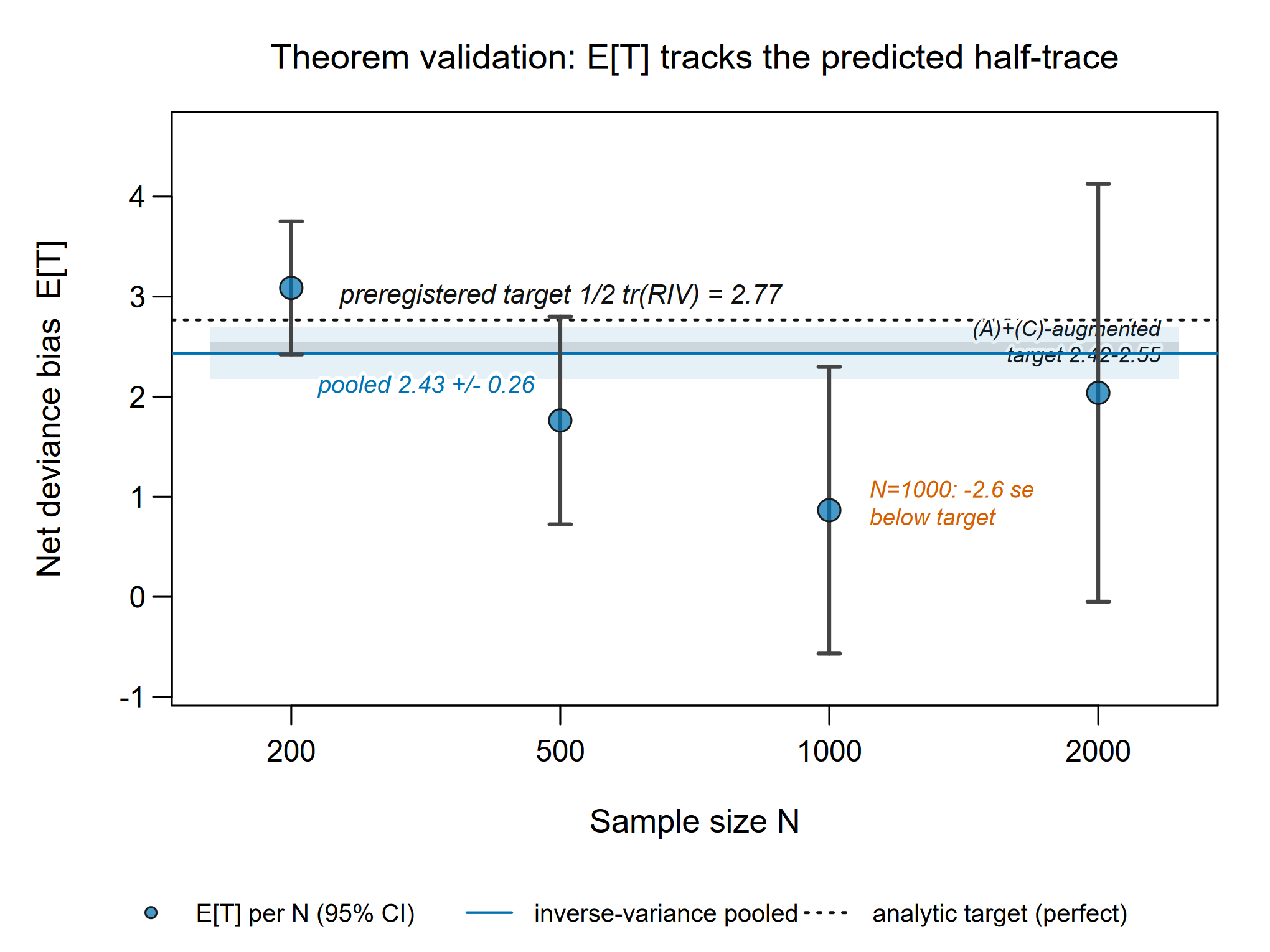
Figure 1. Theorem validation. Each point is the net deviance bias \(\mathbb{E}[T]\) at one sample size with a 95 percent interval, estimated on the analytic arm with 1000 repetitions. The analytic target is the reference: the dotted line marks the preregistered half-trace 2.77, and the shaded band marks the order-one-augmented prediction 2.42 to 2.55. The solid line is the inverse-variance pooled estimate 2.43 ± 0.26, whose interval contains the leading-order target and centers on the band. The \(N = 1000\) cell falls 2.6 standard errors below the leading-order target, the study's one reported miss.
Known scale and sign regime. Holding the covariance known and fitting only the mean collapses the bias to the two values Equation 14 predicts (Figure 2). The deterministic arm returns 0.025 ± 0.018 against a target of zero, while the proper arm returns −0.536 ± 0.018 against \(-\frac{1}{2}\operatorname{tr}(\mathrm{RIV}) = -0.561\). Both arms are within Monte Carlo error of their targets, and the difference between the two arms matches the predicted posterior-draw imputation variance. Imputing from the true model rather than the fitted model reverses the sign of the total, and that sign reversal is what the fitted-model-versus-true-model distinction requires.
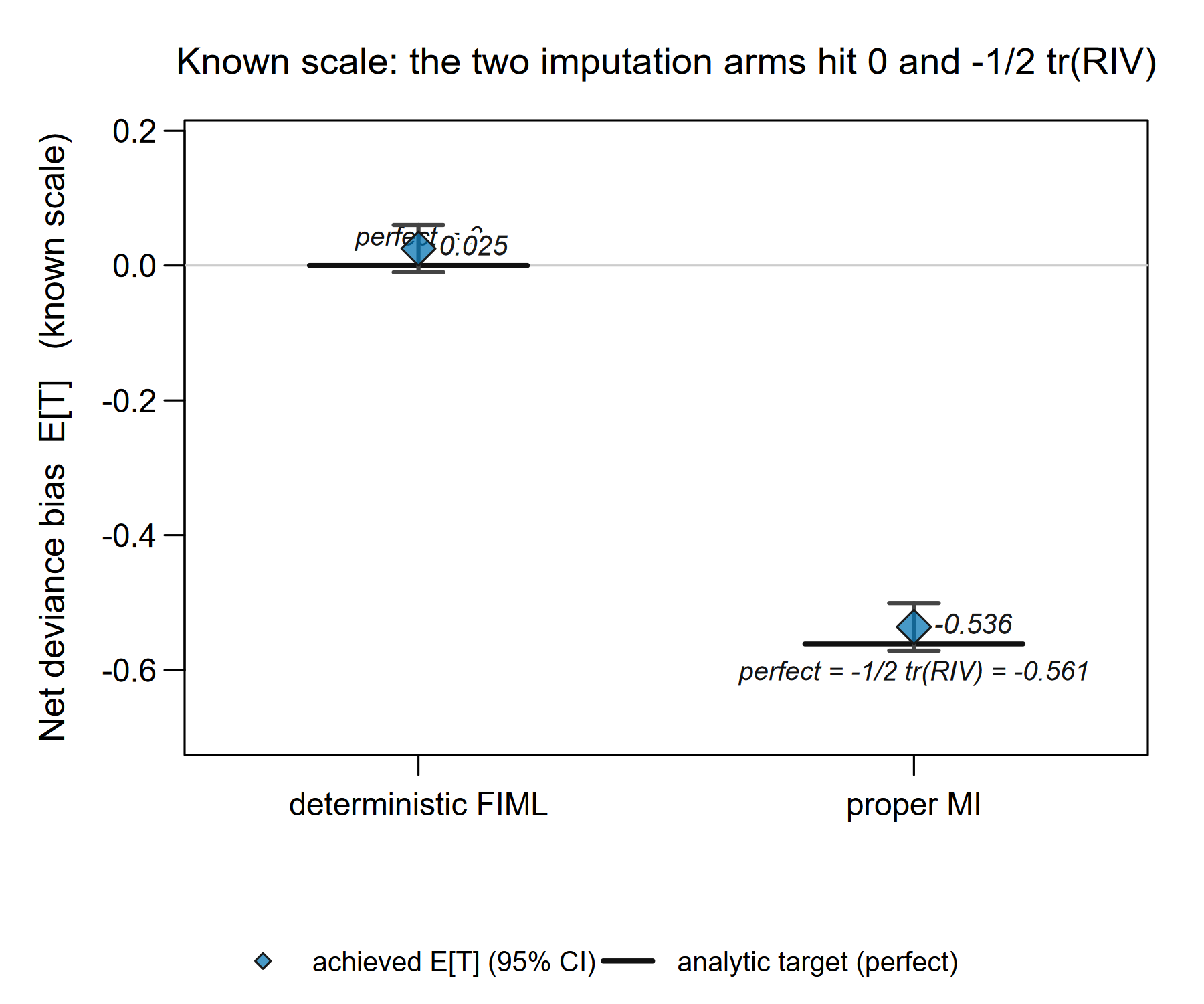
Figure 2. Known scale. The two imputation arms of the known-scale run at \(N = 200\) with \(2 \times 10^5\) repetitions, each with a 95 percent interval. The reference is the pair of analytic targets. The target is zero for the deterministic arm and \(-\frac{1}{2}\operatorname{tr}(\mathrm{RIV}) = -0.561\) for the proper arm. Both arms reach their target within Monte Carlo error.
Likelihood-ratio absorption. A correctly calibrated reference absorbs the differential bias at the null, so the test controls its Type I error (Figure 3). The uncorrected numerator rejects at 0.042 and the additionally corrected numerator at 0.034. Both lie near the nominal 0.05. The corrected one is slightly conservative, as double-counting predicts. Raw power across the alternative is not compared here. The four references reject at different Type I error, so a raw power comparison would be confounded. The size-adjusted power arms are the partial support cited for the power conjecture of Section 7. One scope note travels with this study. Its committed correction arm used the naive trace difference. That difference is about 5 percent from Equation 17 in this near-invariance design and is immaterial here. Still, Equation 17 is the correct general form.
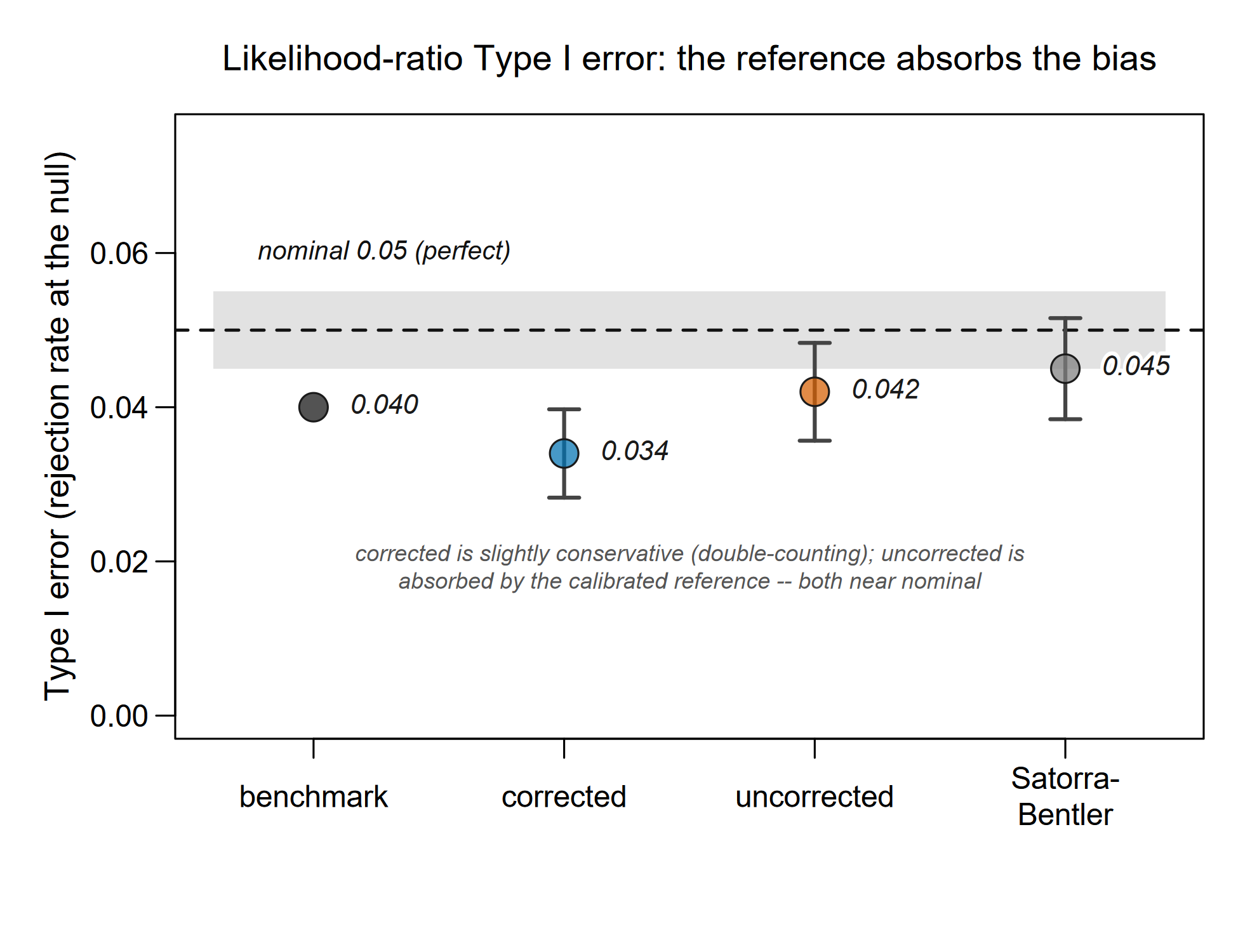
Figure 3. Likelihood-ratio Type I error. The rejection rate at the null for four references at \(N = 200\) with 1000 repetitions and Monte Carlo error bars. The reference is the nominal 0.05 line. The uncorrected numerator lies at 0.042 and the corrected one at 0.034. Both are near nominal. The corrected one is slightly conservative because it double-counts. Raw power across the alternative is not shown. The references reject at different Type I error, so the comparison would be confounded. The size-adjusted power conjecture is treated in the Discussion.
Discrimination of the two formulas. This run uses an adversarial design that makes one coordinate 70 to 79 percent missing. That design separates the two candidate formulas as widely as it allows (Figure 4). The observed differential is 2.64 ± 0.11 at \(N = 500\) and 2.70 ± 0.11 at \(N = 1000\). Both match the projected-trace prediction of 2.64. Correctness rests on that match. The same statistic lies 52 standard errors from the naive trace difference. That gap excludes the naive formula in this engineered cell. That the naive difference always overstates the projected trace is the proved general statement of Proposition 5.2. The size of the gap here reflects the maximal-separation design rather than typical balanced missingness.
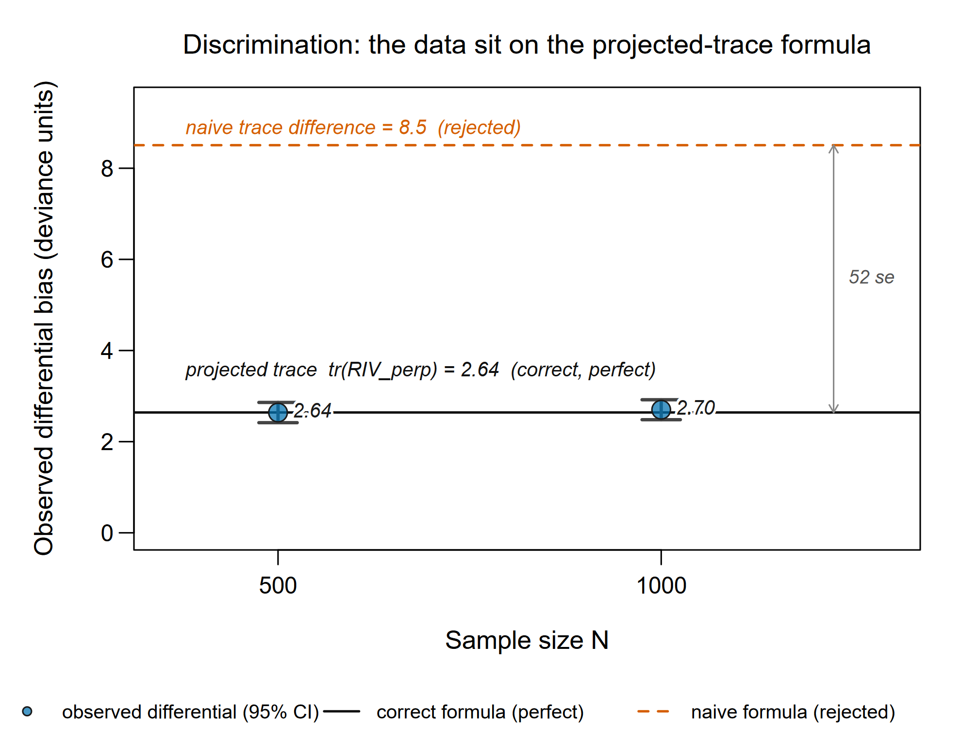
Figure 4. Discrimination. The observed paired differential at two sample sizes with 95 percent intervals, from 2000 repetitions on the heavy-missingness \(\mu_1\) design. The reference is the projected-trace prediction \(\operatorname{tr}(\mathrm{RIV}_\perp) = 2.64\), the solid line. The naive trace difference is the dashed line near 8.5. It is excluded at 52 standard errors in this maximal-separation cell.
Pairing. Comparing the same imputations under both models holds the per-dataset noise at order one (Figure 5). At the null the paired-differential standard deviation stays near 1.5 across \(N = 500, 1000\), and 2000. The single-model figure instead grows from 18.4 to 36.5. At a fixed alternative the square-root-of-\(n\) growth returns, rising to 12.4, 16.8, and 24.9. This is the failure mode the result specifies.
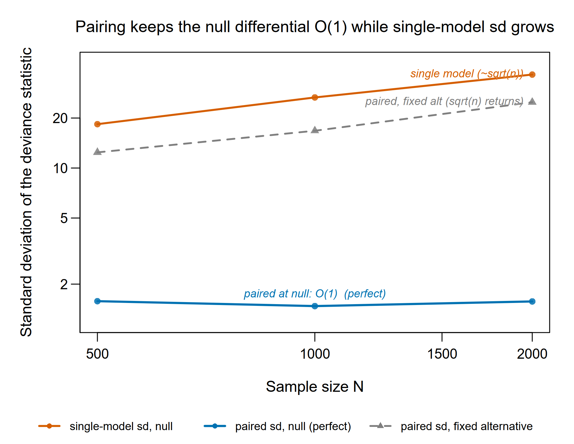
Figure 5. Pairing. Standard deviation of the deviance statistic against sample size, from 2000 repetitions, on a logarithmic scale. The reference is a flat line at order one. The paired differential at the null achieves it, the lower curve. The single-model statistic grows with the sample size. The paired differential at a fixed alternative grows too, the documented limit of pairing.
Selection. The uncorrected criterion favors high-missing-information models, and the correction moves selection back toward the complete-data benchmark (Figure 6). At \(N = 500\) on the deterministic arm, the complete-data benchmark selects the true model at 0.90, while the uncorrected criterion selects it at 0.67 and the corrected criterion at 0.82. In our simulations, every misclassification by the uncorrected criterion fell on the saturated, largest-missing-information candidate, 100% in all sixty cells. This directional pattern was registered for the congenial cells and held in the uncongenial ones as well. Because the candidates are nested and ordered by missing information, the saturated model is the natural destination for any downward-biased deviance, so the error pattern confirms the predicted direction of the bias rather than discriminating the specific decomposition. The recovery is substantial but visibly short of the complete-data benchmark, and that gap is what the distribution-matching ladder was registered to explain.
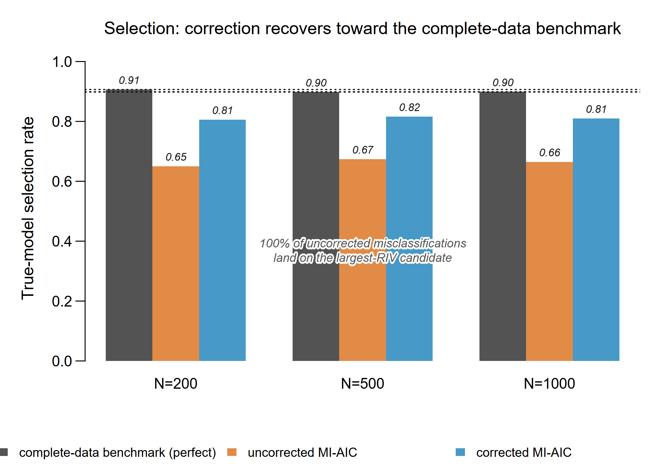
Figure 6. Selection. True-model selection rate by the Akaike criterion at three sample sizes on the non-monotone missing-at-random cell, 2000 repetitions. The reference is the complete-data benchmark, the dashed line and the black bar. The uncorrected criterion lies well below it, and the correction recovers most of the gap. All uncorrected errors fall on the largest-missing-information candidate.
The distribution-matching ladder. Across three levels of signal strength, the stronger constructions recover the complete-data benchmark wherever the errors come from choosing too rich a model, while a residual shortfall remains where selection is hard even with complete data (Figure 7). The true-model selection rates are reported in Table 2, with Monte Carlo standard error near 0.010.
At correlation 0.40 the two-moment and equating arms reach 0.904 and 0.903 against a complete-data benchmark of 0.899; because the differences are within twice the Monte Carlo standard error of about 0.010, both arms are statistically indistinguishable from the benchmark, with a small overshoot the same interval does not resolve. The zero-correlation cell removes 90 percent of the difference between the uncorrected criterion and the benchmark. In the weak-signal cell, by contrast, the benchmark itself drops to 0.820 and no arm passes 0.650. We read that shortfall as a limit of the information in the data rather than as a calibration error, an interpretation the calibration checks below support, although they do not separately decompose it in the weak-signal cell; the residual is a measurement on these designs rather than a theorem.
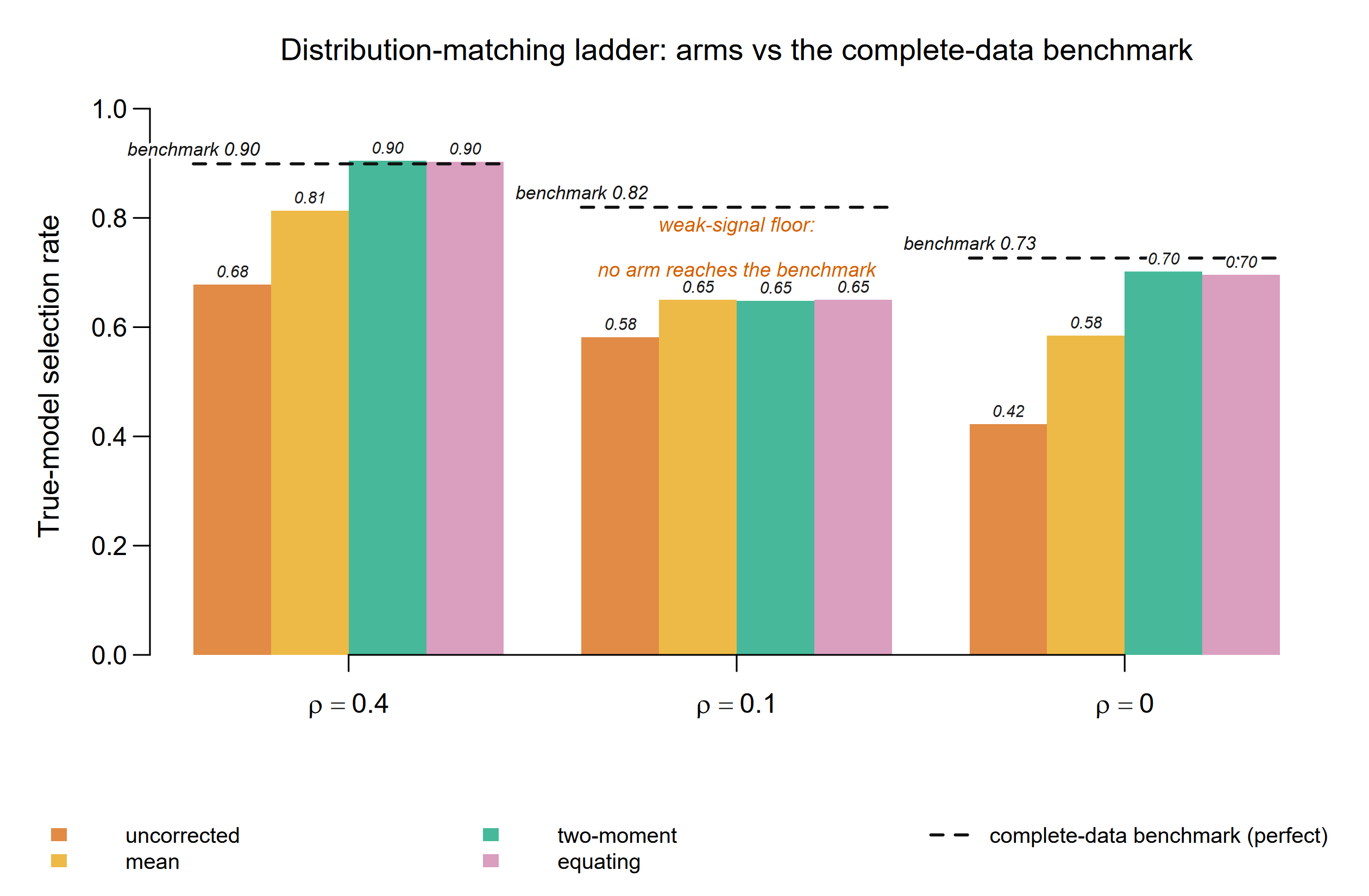
Figure 7. Distribution-matching ladder. True-model selection rate for four constructions in three cells at \(N = 500\) with 2000 repetitions. The reference is the complete-data benchmark, the dashed line above each cell. At \(\rho = 0.40\) the two-moment and equating arms reach the benchmark. At \(\rho = 0.10\) no arm reaches it, the weak-signal shortfall.
Ladder internals. Two internal measurements show why the ladder succeeds (Figure 8). On the true model's anchored statistic the distance to the paired complete-data statistic falls from 0.281 under the uncorrected deviance to 0.018 under equating. Over the same arms the variance ratio falls from 3.18 to near one. The mean correction's paired gap of 0.076 ± 0.100 is a direct confirmation of Equation 17 at four tested directions. On the underfit candidate the noncentral statistic shrinks by its two predicted factors. The two-moment match shrinks it by the factor \(a_k\), predicted near 0.56 and measured at 0.59. Equating shrinks it by \(1/\lambda_{\max}\), predicted near 0.40 and measured at 0.36. The internal validity checks held on every repetition. The spectrum-trace identity held to \(3 \times 10^{-15}\), and the reference inversion never failed in 18,000 evaluations.
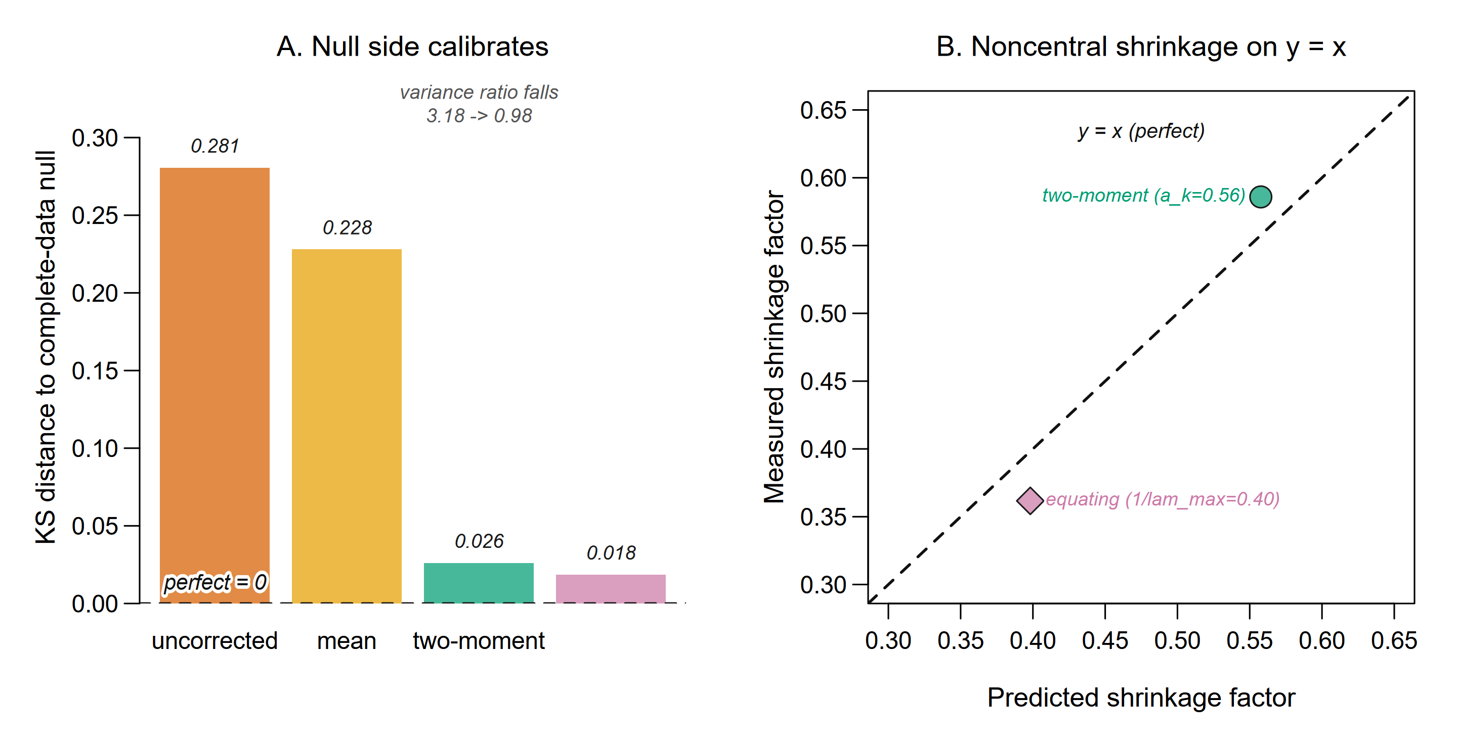
Figure 8. Ladder internals. Left, the null-side Kolmogorov-Smirnov distance to the complete-data statistic across the four arms in the main cell. The reference is zero, approached by the two-moment and equating arms, with the variance ratio falling from 3.18 toward one. Right, the noncentral shrinkage factor measured against predicted on the line \(y = x\). The two-moment and equating points lie on the diagonal.
The structural limits. Three structural checks of Section 5 appear directly in the data. They are the equality case where the naive and projected traces coincide, the cost of the naive moment-map input, and the limit of a per-model map. Table 4 reports them on the selection rates, with Monte Carlo standard error near 0.010.
Two points follow. In this block-diagonal candidate family the naive and projected traces coincide, to \(3.6 \times 10^{-15}\), so the family cannot by itself separate the two trace formulas. The 0.824 against 0.904 gap in the second row is therefore a cost of the naive moment-map input, not evidence about the trace formulas. Where the trace formulas actually do differ, the proof of Proposition 5.2 establishes that the naive trace difference overstates the projected trace, and the non-nested measurement of Figure 9 supplies the measured off-equality case, about 9 percent. The third row is separate again, and it shows that a per-model marginal map cannot calibrate the joint difference distribution.
The non-nested measurement. This study checks three claims at once (Figure 9). The mechanism behind the design-imbalance term is confirmed, the predicted scaling resolves for a dissimilar pair, and the pre-registered prediction for the similar pair stays below resolution. Each candidate's order-one level is large under missing-at-random data, near +2.6 and +2.9 deviance units for the two candidates, but that level collapses under the completely-at-random twin, most sharply for the autoregressive candidate. For the dissimilar diagonal-versus-autoregressive pair the isolated differential resolves at −1.2, lying three and a half standard errors from zero and staying stable across sample sizes. For the similar compound-symmetry-versus-autoregressive pair, by contrast, the differential lies below Monte Carlo resolution. A pilot's apparent value of −2 did not persist in the full run, a failure we report as the pre-registration requires. As a byproduct, the analysis gave the first measured case off the equality condition of Proposition 5.2, where the naive trace difference overstates the exact projected trace by about 9 percent.
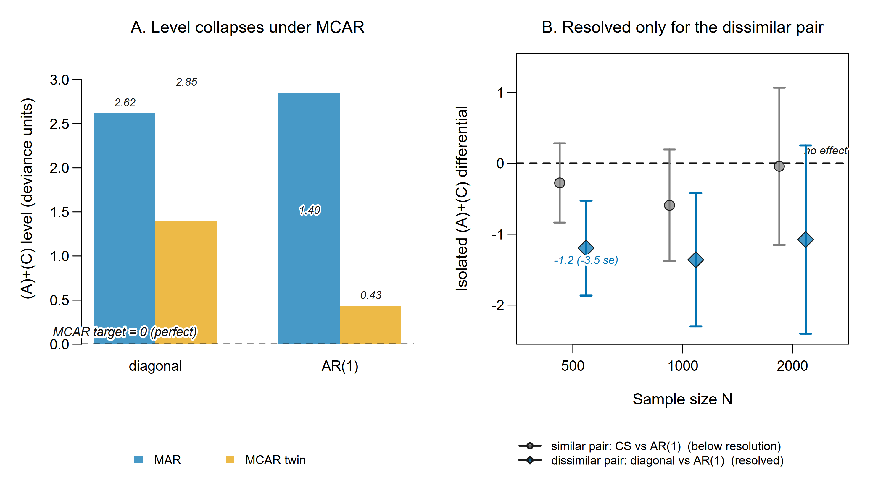
Figure 9. Non-nested measurement. Left, each candidate's order-one level under missing-at-random data and under its completely-at-random twin, dissimilar pair at \(N = 500\) with 20,000 repetitions. The twin's reference is zero, and the level collapses toward it, most sharply for the autoregressive candidate. Right, the isolated design-imbalance differential with 95 percent intervals. The reference is no effect, the line at zero. The similar pair stays on that line, the reported failure, while the dissimilar pair resolves at −1.2.
Engine sensitivity. The bootstrap imputation sampler reproduces the analytic results on the most demanding cells, which indicates the cost of not running data augmentation is small on these designs. Its hardest case is the non-monotone missing-at-random cells with samples as small as \(N = 200\), where the bootstrap approximation is weakest. Even there the sample relative-increase-in-variance trace from the imputation draws matches the observed-data value within 2 to 3 percent, with no widening as the sample grows. Selection also agrees between the analytic arm and the imputation arm within 0.011 on the recovery gap. This robustness is empirical and restricted to the designs studied. The bootstrap sampler is only approximately Bayesian and data augmentation was not run, so a fully Bayesian sampler remains the conservative choice when the fraction of missing information is large (Section 7).
7 Discussion
The scope of the result follows from its own mechanism, and we state that scope first. The deviance optimism that inflates the criteria exists only when the fit estimates a scale or covariance, because only then does the conditional missing-data entropy depend on the estimated parameters; a known-scale, location-only fit has no such bias under deterministic FIML and only \(-\frac{1}{2}\operatorname{tr}(\mathrm{RIV})\) under proper MI, which is why the estimated-scale clause belongs in the statement of the theorem rather than in a footnote. Congeniality is assumed throughout, and what the bias becomes without it (Meng, 1994) is a separate question that this paper does not take up. Beyond these scope conditions, nine specific limits remain, labeled G1 through G9, each stated next to the claim it qualifies together with its evidential standing, and they are followed by one conjecture, three directions, and the answer to the question the paper opened with.
G1. The absolute magnitude of \((A) + (C)\) is not independently determined. This qualifies the theorem. The structural facts are firm. Its sign, its \(O(1)\) order, its exact MCAR vanishing, the closed form Equation 13, and the \(O(1/n)\) order of the correction beyond the leading-order analytic value are all proved. The absolute magnitude is not. The direct Monte Carlo estimates are heavy-tailed and untrended. The variance-reduced estimate of the higher-order remainder is conditional on the analytic anchor it is paired against. Every comparison in this paper therefore uses \((A) + (C)\) only through the better-conditioned paired differential.
G2. The proper-MI carry-over of the likelihood-ratio propositions is structural, not separately measured. This qualifies the likelihood-ratio part of Section 5. The propositions are proved and confirmed for the deterministic-FIML \(\bar{Q}_\infty\). Under proper MI the imputation-side quantities remain common to both fits. This preserves the cancellation arguments. But no dedicated proper-MI replication of the differential experiments exists.
G3. Imputation-engine robustness is empirical and restricted in scope, which qualifies Section 6. On the designs studied, the EMB engine tracks deterministic FIML within the stated tolerances. Exact data augmentation was not run, so nothing here establishes engine-independence beyond those designs.
G4. The weak-signal shortfall is a measurement, not an impossibility proof, and this qualifies the selection part of Section 5. In the weak-signal cell, the residual is information loss as measured through these corrections. No argument here shows that no estimator built from the same observed data could do better.
G5. For dissimilar candidate pairs, a mechanism-independent misspecification \(O(1)\) coexists with the design-imbalance \(O(1)\). This qualifies Proposition 5.4 and its use in selection. The MCAR contrast separates the two in measurement. But they can reinforce or partially offset each other in the net ranking bias a criterion sees. We make no claim that the design-imbalance term dominates every pair.
G6. All instantiation is multivariate normal. This qualifies the theorem. The theorem is stated for general regular likelihoods with an estimated scale. But every constant is verified, symbolically and by simulation, only in the normal family.
G7. The correction's guarantees assume congenial imputation. Uncongeniality is the practical boundary. The imputation model can shrink the cross-block correlations that the analysis estimates. A strong ridge prior does this. When it happens the deviance bias no longer points the way the theory assumes. The sweep includes uncongenial cells, and they show the effect. There the uncorrected criterion already selects the true model more often than the complete-data benchmark, near 0.93 against the benchmark's 0.91. The correction then pushes past the benchmark to about 0.98. That is an overshoot, not a recovery. We registered this behavior as an observational stress test, not as a pass target. It marks where the framework's safety margin ends. In practice it is wise to diagnose congeniality before trusting bias-corrected selection. Practical tools for that diagnosis exist. He and Zaslavsky (2012) give a posterior predictive check that applies the analyst's own target analysis to the completed data and to replicates drawn under the imputation model, and their re-imputation scheme runs on standard imputation software. Bondarenko and Raghunathan (2016) compare observed and imputed values conditional on the response propensity, so an analyst can judge congeniality without knowing the imputation model. Nguyen et al. (2017) review these and related checks for applied use.
G8. BIC carries the same directional bias as AIC, but its own penalty grows with the sample size while AIC's does not, so at the sizes used in the main sweep BIC is already close to the complete-data benchmark before any correction is applied. The corrected criterion is \(\mathrm{BIC}^c_{\mathrm{MI}}(k) = -2\bar{Q}_\infty(\hat{\psi}^*_k) + q_k \log N + \operatorname{tr}(\mathrm{RIV}_k)\): the same trace correction as Equation 21 applied to the same deviance, with BIC's own sample-size-dependent penalty and the complete-data \(N\) in it. At \(N = 200\), uncorrected BIC selects the true model at 0.98 against the benchmark's 1.00, and every one of its rare misclassifications falls on the largest-missing-information candidate, so the correction has little left to recover, closing the gap to 0.99. As a follow-up check outside the pre-registered sweep, we reran the same comparison at \(N = 50\) and \(N = 100\), where BIC's penalty has not yet grown large enough to dominate. There uncorrected BIC's selection rate falls to about 0.75 at \(N = 50\) and 0.94 at \(N = 100\), against benchmarks of 0.93 and 0.99, and the correction recovers proportionally more of the gap. The concentration on the largest-missing-information candidate weakens in step. Only about 0.55 to 0.62 of BIC's more frequent errors at \(N = 50\) fall on that candidate, rising to about 0.88 to 0.89 at \(N = 100\) and to essentially all of them by \(N = 200\). So the concentration pattern reported above for AIC is, for BIC, a property of large samples, tied to a penalty that grows with \(N\), and not a law that holds at every size studied. In practice the correction should be expected to matter most for BIC where its own penalty has not yet reached that regime, and any BIC-based comparison at a small sample should be read with that limit in mind.
G9. A first check outside the normal family exposed an error in our own registration before it sharpened the theory, and we report it in that order. We registered a Gamma model as the estimated-scale exemplar and a Bernoulli model as the known-scale exemplar. The registered Bernoulli prediction for the genuine posterior draw was approximately −0.5 times the trace; the measured value was +0.63 (se 0.16), about seven standard errors away and of the opposite sign, and the plug-in arm missed its registered target of approximately 0 by about five standard errors. The registration had treated the absence of a named dispersion parameter as the known-scale condition, but the collapse actually requires the family's conditional missing-data entropy to stay flat in the estimated parameter, and the binary entropy is not flat, because its derivative is the negative logit. After the miss we derived what a canonical-link model should show, rather than re-scoring against an assumed value. Under response-only MCAR missingness the two order-one design terms in the theorem's proof cancel exactly for any canonical link, so the plug-in bias is the general \(+\frac{1}{2}\) trace value plus a base-measure term. That term is zero for Bernoulli and moves Poisson to a derived +0.10. Because this derivation was produced after the miss, its predictions were pre-registered and then run blind. The Bernoulli plug-in reaches an asymptote of +0.51 ± 0.04 across an \(N\)-scan against the derived +0.5, and the earlier +0.85 at \(N\)=200 proves to have been Monte-Carlo noise around a true +0.52. A Poisson model, simulated here for the first time only after its target was fixed, measures +0.11 ± 0.03 against its derived +0.10. A Student-t location model with fixed scale, a genuine known-scale family, measures +0.02 ± 0.05 for the plug-in and −0.48 ± 0.05 for the posterior draw against the derived 0 and −0.5, so the known-scale collapse now has a check outside the normal family. The superseded Bernoulli draw value also carried a fixed imputation seed across repetitions, which its quoted standard error did not reflect. The Gamma result stays directional (+0.32 ± 0.20 against the predicted one half), because its log link is not canonical and the new argument does not cover it. What G6 keeps is therefore sharper but real. Membership in the two cases is decided by the entropy-gradient condition and, for canonical links, by the base measure, not by the family's name. Non-canonical links remain underived.
One question is left as a conjecture, and we label it as one. We conjecture that the bias-corrected likelihood-ratio comparison dominates its uncorrected counterpart in power uniformly; the preregistered likelihood-ratio study's power arms provide partial support (Section 6), but we state no theorem.
Three directions seem most worth pursuing. The first is covariate shift. The concluding section of Shimodaira and Maeda (2018) names the combination of a missing mechanism with other sampling mechanisms as future work. The design-imbalance term derived here is nonzero exactly when the missing and observed units differ on the conditioning variables. This is a step into that program. The weighting machinery exists (Shimodaira, 2000). The second is an exact-engine replication. Running the main studies under data augmentation would convert G3 from an empirical tolerance into a tested equivalence. The third is the calibration program beyond per-model null maps. De-shrinkage of estimated noncentrality and joint calibration of score vectors across candidates are left to future work. So is the extension beyond the normal family.
The paper closes where it began, with the replication principle. The question was whether an analyst working from multiply imputed data reaches the same conclusions, as often, as the analyst who never lost the data. The answer now has three parts. The first part concerns the criterion itself. The answer is yes. After correction, a deviance or information criterion computed from imputed data means what its complete-data counterpart means, on average, at any signal strength. The second part concerns decisions when the competing models fit alike. The answer is again yes. There, corrected selection and calibrated tests behave as they would have with complete data. The third part concerns decisions when one model truly fits better. There the answer is no. The missing data carried part of the evidence. Less information means less power. No correction studied here manufactures the lost evidence back. In practical terms the advice is short: correct the criterion, or match its null distribution, and then trust the result the way complete-data results are trusted, subject to the stated conditions. The one exception is where the comparison was close enough that the missing data could have decided it. There, the honest answer is that the data no longer say.
Two implications for applied practice follow. The first is statistical. When the aim is to rank models on imputed data, and no calibrated reference distribution already absorbs the bias, add the per-candidate trace correction before reading off the result. Information-criterion selection is the main such case. The exception is a calibrated likelihood-ratio test, where the reference distribution already carries the null mean, so a numerator correction applied on top would double-count and should be left out. For a nested comparison without a calibrated reference, the relevant bias is the missing information in the tested directions alone, not the difference of the candidates' separate trace corrections. The second implication is about method. An applied team deciding whether to rely on a human-prompted AI derivation can ask for the same evidence required here. That evidence is citations checked against their sources, independent symbolic checks, preregistered numerical criteria with their failures reported, adversarial review by a separate model, and a reproducible record. What makes such a result safe to use is the standard it meets, not the name of the system that produced it.
A final word on the workflow, held to the same standard as everything it produced. Three catches are on the record. The protocol caught a sign error that eight of nine blind re-derivations shipped, caught a wrong shortcut in an early entropy-gradient argument, and forced every failed prediction into Section 6. The cost is also visible. Claims arrived slower, hedged to their grade, and two preregistered predictions were given up rather than salvaged. What it cannot catch was stated in Section 4 and bears repeating once. It cannot catch errors shared across model lineages, misreadings of real sources, or designs that answer the wrong question reproducibly. Whether this workflow generalizes beyond one paper is asserted, not demonstrated. What it leaves behind is a public record. The decision log, the preregistrations with their amendments, the verification checks, and the session transcripts are all published. So the assertion can be tested by someone other than its authors.
8 References
- Akaike, H. (1974). A new look at the statistical model identification. IEEE Transactions on Automatic Control, 19(6), 716–723. https://doi.org/10.1109/TAC.1974.1100705
- Asparouhov, T., & Muthén, B. (2006). Robust Chi Square Difference Testing with Mean and Variance Adjusted Test Statistics: Webnote 10. https://doi.org/http://www.statmodel.com/examples/webnotes/webnote10.pdf
- Asparouhov, T., & Muthén, B. (2010). Simple Second Order Chi-Square Correction.
- Bondarenko, I., & Raghunathan, T. (2016). Graphical and numerical diagnostic tools to assess suitability of multiple imputations and imputation models. Statistics in Medicine, 35(17), 3007–3020. https://doi.org/10.1002/sim.6926
- Cavanaugh, J. E., & Shumway, R. H. (1998). An Akaike information criterion for model selection in the presence of incomplete data. Journal of Statistical Planning and Inference, 67(1), 45–65. https://doi.org/10.1016/S0378-3758(97)00115-8
- Chan, K. W. (2022). General and feasible tests with multiply-imputed datasets. The Annals of Statistics, 50(2). https://doi.org/10.1214/21-AOS2132
- Chan, K. W., & Meng, X.-L. (2022). Multiple Improvements of Multiple Imputation Likelihood Ratio Tests. Statistica Sinica. https://doi.org/10.5705/ss.202019.0314
- Claeskens, G., & Consentino, F. (2008). Variable Selection with Incomplete Covariate Data. Biometrics, 64(4), 1062–1069. https://doi.org/10.1111/j.1541-0420.2008.01003.x
- Consentino, F., & Claeskens, G. (2010). Order selection tests with multiply imputed data. Computational Statistics & Data Analysis, 54(10), 2284–2295. https://doi.org/10.1016/j.csda.2010.04.009
- Davies, R. B. (1980). Algorithm AS 155: The Distribution of a Linear Combination of \(\chi^2\) Random Variables. Applied Statistics, 29(3), 323. https://doi.org/10.2307/2346911
- Dempster, A. P., Laird, N. M., & Rubin, D. B. (1977). Maximum Likelihood from Incomplete Data Via the EM Algorithm. Journal of the Royal Statistical Society Series B: Statistical Methodology, 39(1), 1–22. https://doi.org/10.1111/j.2517-6161.1977.tb01600.x
- Enders, C. K. (2025). Missing data: An update on the state of the art. Psychological Methods, 30(2), 322–339. https://doi.org/10.1037/met0000563
- He, Y., & Zaslavsky, A. M. (2012). Diagnosing imputation models by applying target analyses to posterior replicates of completed data. Statistics in Medicine, 31(1), 1–18. https://doi.org/10.1002/sim.4413
- Hens, N., Aerts, M., & Molenberghs, G. (2006). Model selection for incomplete and design-based samples. Statistics in Medicine, 25(14), 2502–2520. https://doi.org/10.1002/sim.2559
- Honaker, J., King, G., & Blackwell, M. (2011). Amelia II: A Program for Missing Data. Journal of Statistical Software, 45(7). https://doi.org/10.18637/jss.v045.i07
- Imhof, J. P. (1961). Computing the distribution of quadratic forms in normal variables. Biometrika, 48(3-4), 419–426. https://doi.org/10.1093/biomet/48.3-4.419
- Kenward, M. G., & Molenberghs, G. (1998). Likelihood Based Frequentist Inference When Data Are Missing at Random. Statistical Science, 13(3), 236–247. https://www.jstor.org/stable/2676702
- Kolen, M. J., & Brennan, R. L. (2014). Test equating, scaling, and linking: Methods and practices (Third edition). Springer.
- Meng, X.-L. (1994). Multiple-Imputation Inferences with Uncongenial Sources of Input. Statistical Science, 9(4). https://doi.org/10.1214/ss/1177010269
- Meng, X.-L., & Rubin, D. B. (1991). Using EM to obtain asymptotic variance-covariance matrices: The SEM algorithm. Journal of the American Statistical Association, 86(416), 899–909. https://doi.org/10.1080/01621459.1991.10475130
- Meng, X.-L., & Rubin, D. B. (1992). Performing likelihood ratio tests with multiply-imputed data sets. Biometrika, 79(1), 103–111. https://doi.org/10.1093/biomet/79.1.103
- Nguyen, C. D., Carlin, J. B., & Lee, K. J. (2017). Model checking in multiple imputation: An overview and case study. Discover Public Health, 14(1), 8–12. https://doi.org/10.1186/s12982-017-0062-6
- Nielsen, S. F. (2003). Proper and Improper Multiple Imputation. International Statistical Review, 71(3), 593–607. https://doi.org/10.1111/j.1751-5823.2003.tb00214.x
- Orchard, T., & Woodbury, M. A. (1972). A Missing Information Principle: Theory and Applications.
- Rubin, D. B. (1976). Inference and missing data. Biometrika, 63(3), 581–592. https://doi.org/10.1093/biomet/63.3.581
- Rubin, D. B. (1987). Multiple imputation for nonresponse in surveys. Wiley.
- Satorra, A., & Bentler, P. M. (2010). Ensuring Positiveness of the Scaled Difference Chi-square Test Statistic. Psychometrika, 75(2), 243–248. https://doi.org/10.1007/s11336-009-9135-y
- Schafer, J. L. (1997). Analysis of incomplete multivariate data (1st ed). Chapman & Hall/CRC.
- Schafer, J. L., & Graham, J. W. (2002). Missing data: Our view of the state of the art. Psychological Methods, 7(2), 147–177. https://doi.org/10.1037/1082-989X.7.2.147
- Schomaker, M., & Heumann, C. (2014). Model selection and model averaging after multiple imputation. Computational Statistics & Data Analysis, 71, 758–770. https://doi.org/10.1016/j.csda.2013.02.017
- Shimodaira, H. (2000). Improving predictive inference under covariate shift by weighting the log-likelihood function. Journal of Statistical Planning and Inference, 90(2), 227–244. https://doi.org/10.1016/s0378-3758(00)00115-4
- Shimodaira, H., & Maeda, H. (2018). An information criterion for model selection with missing data via complete-data divergence. Annals of the Institute of Statistical Mathematics, 70(2), 421–438. https://doi.org/10.1007/s10463-016-0592-7
- Tierney, L., & Kadane, J. B. (1986). Accurate approximations for posterior moments and marginal densities. Journal of the American Statistical Association, 81(393), 82–86. https://doi.org/10.1080/01621459.1986.10478240
- Vaart, A. W. V. D. (1998). Asymptotic Statistics (1st ed.). Cambridge University Press. https://doi.org/10.1017/CBO9780511802256
- van Buuren, S. (2018). Flexible Imputation of Missing Data, Second Edition (2nd ed.). Chapman and Hall/CRC. https://doi.org/10.1201/9780429492259
- Vuong, Q. H. (1989). Likelihood Ratio Tests for Model Selection and Non-Nested Hypotheses. Econometrica, 57(2), 307. https://doi.org/10.2307/1912557
- Wei, G. C. G., & Tanner, M. A. (1990). A Monte Carlo Implementation of the EM Algorithm and the Poor Man's Data Augmentation Algorithms. Journal of the American Statistical Association, 85(411), 699–704. https://doi.org/10.1080/01621459.1990.10474930
- Wilks, S. S. (1938). The Large-Sample Distribution of the Likelihood Ratio for Testing Composite Hypotheses. The Annals of Mathematical Statistics, 9(1), 60–62. https://doi.org/10.1214/aoms/1177732360
- Wood, A. M., White, I. R., & Royston, P. (2008). How should variable selection be performed with multiply imputed data? Statistics in Medicine, 27(17), 3227–3246. https://doi.org/10.1002/sim.3177
Table 1. The studies of this section mapped to the claims they test. Each row names a claim from Section 5, the analytic result behind it, the study that tests it, the outcome with its exhibit, and the assessment against the pre-registered pass criterion.
| Claim tested | Analytic basis | Study | Result | Verdict |
|---|---|---|---|---|
| The averaged log-likelihood overstates its complete-data counterpart by \(\frac{1}{2}\operatorname{tr}(\mathrm{RIV}) + (A)+(C)\) | Theorem 5.1 | Theorem validation | pooled 2.43 ± 0.26, centered on the augmented band 2.42 to 2.55 (Figure 1) | pass (pooled criterion met); the \(N = 1000\) cell missed, reported |
| Known-scale collapse: bias 0 under deterministic FIML, \(-\frac{1}{2}\operatorname{tr}(\mathrm{RIV})\) under proper MI | Equation 14 | Known scale and sign regime | 0.025 ± 0.018 and −0.536 ± 0.018 against targets 0 and −0.561 (Figure 2) | pass |
| Imputing from the true model reverses the sign of the total | the conditioning fork at Equation 8 | Known scale and sign regime | the total reverses sign, as the fitted-versus-true-model distinction requires (reported with Figure 2) | pass |
| A calibrated reference absorbs the null bias, so correcting the numerator on top double-counts | Equation 20 | Likelihood ratio | Type I error 0.042 uncorrected and 0.034 corrected, near the nominal 0.05 (Figure 3) | pass (corrected arm conservative, as double-counting predicts) |
| The differential bias at the null is \(\operatorname{tr}(\mathrm{RIV}_\perp)\), not the naive trace difference | Proposition 5.1, Proposition 5.2 | Formula discrimination | 2.64 ± 0.11 and 2.70 ± 0.11 against the predicted 2.64; the naive 8.5 excluded at 52 standard errors (Figure 4) | pass |
| Pairing holds the differential's noise at \(O(1)\) | Proposition 5.3 | Pairing | null sd near 1.5 and flat, against 18.4 to 36.5 for a single model; the fixed alternative reverts (Figure 5) | pass |
| Uncorrected MI-AIC favors the largest-RIV candidate, and the trace correction restores selection | Theorem 5.1, Equation 21 | Selection sweep | 0.67 uncorrected, 0.82 corrected, benchmark 0.90 at \(N = 500\); 100% of misclassifications on the largest-RIV candidate (Figure 6) | pass (both registered conditions) |
| The null side calibrates map by map, and noncentral statistics shrink by predictable factors | the three maps of Section 5 | Distribution-matching ladder | two-moment and equating arms reach 0.904 and 0.903 against the benchmark 0.899; shrinkage 0.59 and 0.36 against predicted 0.56 and 0.40 (Table 2, Figure 8) | pass (all three registered conditions); the weak-signal shortfall was itself the registered prediction |
| Block-diagonal families fall at the equality case, and per-model maps cannot calibrate a difference | Proposition 5.2; the structural limits of Section 5 | Distribution-matching ladder | equality to \(3.6 \times 10^{-15}\); naive-input cost 0.824 against 0.904; difference law 6.10 and 5.99 against 10.00 and 7.10 (Table 4) | pass (structural predictions matched) |
| The design-imbalance differential decouples only for separated candidates and grows with dissimilarity | Proposition 5.4 | Non-nested measurement | the dissimilar pair resolves at −1.2 (3.5 standard errors); the similar pair stays below resolution (Figure 9) | mixed: mechanism and dissimilar pair pass; the similar-pair prediction failed |
| The bootstrap engine tracks the analytic arm, bounding the cost of not running data augmentation | the G3 scope statement of Section 7 | Engine sensitivity | tr(RIV) within 2 to 3 percent; selection within 0.011 | within stated tolerances (empirical bound, no registered criterion) |
Table 2. True-model selection rates across the distribution-matching ladder. Rate of selecting the true model for each construction in three signal cells at \(N = 500\) with 2000 repetitions; Monte Carlo standard error near 0.010.
| Cell | complete-data | uncorrected | mean | two-moment | equating |
|---|---|---|---|---|---|
| \(\rho = 0.40\) | 0.899 | 0.678 | 0.814 | 0.904 | 0.903 |
| \(\rho = 0.10\) | 0.820 | 0.582 | 0.650 | 0.648 | 0.650 |
| \(\rho = 0\) (no signal) | 0.727 | 0.422 | 0.585 | 0.702 | 0.696 |
Table 4. Structural checks of the derivations seen in the selection rates. Each row pairs a structural prediction with its measured value; Monte Carlo standard error near 0.010.
| Structural limit | reference | achieved |
|---|---|---|
| block-diagonal family, naive vs projected trace | exact equality | agree to \(3.6 \times 10^{-15}\) |
| off-equality moment map, main-cell rate | complete-data 0.899 | naive input 0.824, correct input 0.904 |
| per-model map, equated difference mean and sd | complete-data 10.00 and 7.10 | 6.10 and 5.99 |

No comments yet. Be the first to comment!