We present a qualitative case study of a human-supervised team of specialized AI agents supporting an astronomy research project. The Bot Spectroscopist team, described in the project record as operating through Grok Bot powered by xAI Grok, divided work among orchestration, numerical implementation, data curation, spectroscopy critique, literature search, figure preparation, manuscript editing, and reviewer. Human decisions determined scientific scope, model changes, and manuscript inclusion. The scientific application is CondGen, a deterministic label-to-spectrum network extending our previous work to five individual elemental abundances. The reported CondGen baseline assessment achieved a mean absolute error (MAE) of 0.003681 in continuum-normalized flux when reconstructing synthetic spectra. The bot team also identified a limitation in the cool-star magnesium response through its abundance diagnostics. Building on existing data and notebooks, the AI team completed the reported analysis, figure preparation, and manuscript-drafting tasks in less than a week through human prompting and exchanges among agents. We retrospectively estimate that comparable work by a professor-led team of researchers or students would typically span approximately one academic semester. The study illustrates task delegation, bot team work, artifact exchange, and correction under human supervision.
1. Introduction
Scientific research commonly involves a connected sequence of tasks: defining a problematic, preparing data, implementing methods, checking results, displaying figures, interpreting failures, and communicating conclusions. AI agents can assist across that sequence because they can use tools, exchange intermediate artifacts, and return decisions to a human researcher. Recent work on AI for science and multiagent systems motivates studying how this organization functions in practice, including its limits [1–4]. Astronomy provides a suitable setting because computational analysis already depends on substantial software and data infrastructure [5,6].
In this manuscript we discuss how a team of specialized AI agents, acting as research group (informally named Bot Spectroscopist), were coordinated to carry out interconnected technical and writing tasks, how their outputs were challenged, and where human decisions remained necessary. We reconstruct four episodes from an orchestrator-prepared retrospective record supplied by us. The record describes short task assignments, artifact handoffs, critiques, and approvals rather than extended scientific dialogue. This record provides a qualitative process account, with explicit limits on what can be verified or measured from that source.
The specialized AI agents were tasked with determining abundance-conditioned generation of stellar spectra using a algorithm that they named CondGen. The research continues our existing spectroscopy research program: an autoencoder and parameter-to-latent model for Gaia RVS spectra [7], followed by an optical conditional variational autoencoder (CVAE) [8]. The present target is a deterministic dense network conditioned on effective temperature \(T_{\rm eff}\), surface gravity \(\log g\), projected rotational velocity \(v_e \sin i\), microturbulence \(\xi_t\), and five individual abundances: [Mg/H], [Sc/H], [Ti/H], [Cr/H], and [Fe/H]. These are the nine input dimensions and are used as features to predict the output spectrum.
This scientific task is useful for this workflow study because it combines a substantial synthetic database, model evaluation, abundance-sensitive diagnostics, and manuscript production. Chemically peculiar stars, such as Am/Fm, motivate treating individual metals rather than only bulk metallicity; the selected elements also connect to our earlier A/Am and AFGK analyses [9,10]. Previous methods, such as The Payne and its extensions, predict stellar spectra from atmospheric parameters and individual elemental abundances. These methods provide the scientific background for our CondGen case study [11–13]. Here, generation means predicting a synthetic spectrum from specified stellar parameters and elemental abundances.
This case study builds on our previous research on generating synthetic stellar spectra. Our published studies provide the scientific foundation for CondGen, while the present project examines how a team of AI agents can contribute to the research process under human supervision. The numerical assessments, diagnostic figures, and architecture comparisons presented here illustrate the tasks performed by the agents and the scientific decisions that followed their analysis and review.
The CondGen model uses the nine inputs specified from the outset: four atmospheric parameters and five individual elemental abundances. Resolving power is fixed as a property of the database and is not an additional input. The Orchestrator's summary describes how the bots organized the numerical work and reviewed the resulting assessments. Section 6.1 identifies the source and purpose of the reported baseline diagnostics and exploratory architecture comparisons.
The scientific task is to predict a synthetic spectrum from specified stellar parameters and elemental abundances. Training and evaluation use computationally generated spectra. Estimating abundances from a spectrum, the reverse problem, and applying the method to telescope observations are outside the scope of this study and remain directions for future work.
1.1. Scope and intent of this paper
The primary contribution is a documented case study of research organization using specialized AI agents under human supervision. CondGen supplies the scientific tasks through which delegation, critique, correction, and approval can be examined. The paper does not claim a new state of the art in stellar spectroscopy or present a controlled comparison of speed, cost, or accuracy against alternative team arrangements. Its broader significance lies in illustrating how AI agents can work together as a coordinated research team, supporting tasks that extend from numerical implementation and scientific analysis to figure preparation and manuscript development. Although demonstrated through an astrophysical application, this approach has potential relevance to other research fields in which progress depends on combining different forms of expertise and reviewing intermediate results. The case study therefore offers a practical example of an emerging direction in research: collaboration among human researchers and specialized AI agents. Such collaboration may become an increasingly important part of scientific practice, with researchers defining the questions, exercising scientific judgment, and retaining responsibility for the conclusions.
Part A (Section 2) describes the team, its operating method, and the decisions that illustrate collaboration. Appendix A provides the sequential workflow account. Part B (Sections 3–6) describes the scientific case study, its model design, and the reported project assessments. The Discussion and Conclusion assess what this case supports and what remains unverified.
Part A: AI-team workflow and collaboration evidence.
2. AI-assisted research workflow
To investigate how AI agents could support a research project as a coordinated team, we organized the Bot Spectroscopist team around complementary research responsibilities. These included numerical implementation, data preparation, scientific critique, literature searches, figure production, manuscript editing, reproducibility checks, and astronomy reviewer. An Orchestrator coordinated the specialist assignments and served as the main point of interaction between us and the team.
The division of responsibilities reflected the different activities required to develop and communicate the CondGen case study. Numerical outputs prepared by one specialist could be examined by another, converted into figures, and incorporated into the manuscript. We supplied the scientific objectives and existing research materials, guided the work, and reviewed the resulting outputs. We first introduce the team and its responsibilities, then explain how assignments, communication, and review connected those responsibilities.
2.1. Team setup and specialist roles
The team comprised an Orchestrator and eight specialist roles. The project record identifies the platform as Grok Bot powered by xAI Grok. Team setup consisted of organizing the research work around named responsibilities: coordination, computation, data management, scientific criticism, literature support, visualization, writing, and reproducibility. In this account, a bot's specialization refers to its assigned function within the project. The available record describes this division of work but does not include the complete instructions or configuration used to instantiate each role.
Orchestrator. The Orchestrator connected our research objectives to the specialists' tasks. It proposed milestones, incorporated our decisions, assigned work, and collected the resulting outputs and review comments. When a concern required a scientific or editorial decision, it brought that concern back to us and communicated the agreed next step to the relevant specialists. Its central responsibility was to maintain coordination across the project.
Python/Jupyter Specialist. This bot handled the computational work in notebooks, including model evaluation, diagnostic calculations, short architecture comparisons, and training when authorized. Its outputs included performance measurements, spectral predictions, and model or parameter information needed for figures. These outputs supplied material for scientific review by the Critic and visual presentation by the Artist. The evaluation-protocol correction discussed below illustrates why numerical execution and review were connected.
Data Curator. The Curator's assigned role concerned the organization and description of the numerical inputs: the database schema, training and evaluation partitions, and preprocessing records such as scalers. These records were intended to help the Python/Jupyter Specialist use the appropriate data and transformations when evaluating a model. The role addressed the consistency and traceability of inputs on which subsequent calculations depended; its involvement was task-dependent.
Spectroscopy Domain Critic. The Critic examined spectral diagnostics and assessed whether the accompanying scientific claims were supported. It could return concerns to the Python/Jupyter Specialist for a numerical check, to the Artist for a presentation change, or to the Editor for revised wording. The bot team identified the adverse cool-star Mg response in the abundance diagnostics, and the Critic challenged its presentation as evidence of physical fidelity. We retained responsibility for deciding how such concerns affected the interpretation and reporting of results.
Literature Scout. The Scout supported the research context and bibliography by locating relevant publications and checking citation information. It supplied references and bibliographic corrections to the Editor for integration into the manuscript. Its responsibility concerned the literature supporting the study and the accuracy of its citation records.
Figure Artist. The Artist converted numerical outputs and model specifications into diagrams and diagnostic figures. It used information supplied by the Python/Jupyter Specialist to label stellar parameters, depict the architecture, and present spectral comparisons. It then passed figure files to the Editor and revised presentation problems identified during review, including overlapping labels and figure borders. This role connected the computational results to their visual communication.
LATEX Editor. The Editor assembled text, references, tables, and figures into the Overleaf manuscript. It integrated material supplied by the other specialists, applied agreed revisions, and checked figure inclusion and compilation. The role required coordination with the Scout for references, the Artist for figures, and the Critic for the wording of scientific claims. The assembled document was returned for review and further author decisions.
Reproducibility Auditor. The Auditor's assigned responsibility was to examine the organization of research outputs and the records needed to regenerate them. The workflow account reports packaging and figure-regeneration checks. This role complemented the Critic's examination of scientific interpretation by focusing on whether the supporting materials and production steps could be traced. Its involvement was task-dependent, and the reported checks do not by themselves establish independent reproduction of the numerical results.
Expert Spectroscopy Reviewer. This role was reserved for reviewing the assembled manuscript when assigned. Its remit covered the scientific argument and presentation across the document, complementing the Domain Critic's checks of particular diagnostics and claims during production. It returned revision recommendations to the Orchestrator and us. The account describes the Reviewer as otherwise held in standby, so its inclusion in the roster does not imply continuous participation or an independent external peer review.
Table 1 provides a compact reference to these responsibilities and the exchanges connecting them. The roles were used according to the needs of each task; the record does not establish that every specialist was active throughout the project.
Table 1. Roles for the Bot Spectroscopist team and their interfaces. Roles describe delegated responsibilities; final scientific and publication decisions remained human.
| Role | Reported responsibility | Handoff or decision interface |
|---|---|---|
| Orchestrator | Propose milestones; assign scoped tasks; collect outputs | Human approval before model changes or manuscript insertion |
| Python/Jupyter Specialist | Notebook execution, model evaluation, training | Evaluation outputs and parameter information to Critic and Artist |
| Data Curator | Database schema, split and scaler records | Inputs and provenance for numerical work |
| Spectroscopy Domain Critic | Check spectral diagnostics and claim wording | Concerns returned to Python, Artist, or Editor; authors decide inclusion |
| Literature Scout | Literature searches and bibliography corrections | Source records and citation material to Editor |
| Figure Artist | Prepare figures and parameter labels | Figure paths to Editor; numerical values supplied by Python |
| LATEX Editor | Integrate text, references, and figures | Compiled document returned for review |
| Reproducibility Auditor | Check packaging and regeneration records | Reported audit outcomes and remaining gaps |
| Expert Spectroscopy Reviewer | Review the assembled manuscript when assigned | Revision recommendations to Orchestrator and authors |
2.2. Human direction and research lineage
We, the human authors, supplied the scientific problem, synthetic spectral database, prior notebooks, and CondGen research lineage, drawing on earlier spectral-generation work [7,8]. The agents contributed implementation, evaluation, literature work, testing, figures, and draft text within that existing research program, reviewing, and looping in order to generate the final document.
The bot team contributed to the scientific assessment by identifying a limitation in the model's cool-star magnesium response. The Spectroscopy Domain Critic challenged the interpretation of this diagnostic, and the finding was communicated through the Orchestrator. We decided to retain the diagnostic in the manuscript and report the limitation explicitly. We also approved presenting the architecture comparisons as exploratory tests supporting model selection, established AI teamwork as the manuscript's central focus, and authorized training with nine inputs. These examples illustrate complementary contributions: the agents performed analyses and raised scientific concerns, while we guided the research direction and made decisions about interpretation and reporting.
The authors retain responsibility for the results, interpretation, and final text. However, we question the fact if AI systems should be disclosed only as tools rather than listed as authors [14–17].
2.3. Communication and coordination
The operating sequence reported in the workflow account was: the Orchestrator proposed a milestone, we approved or changed it, and the Orchestrator then assigned work to specialists. The milestones distinguished training, evaluation, and manuscript preparation. Likewise, manuscript passages could be discussed in chat before permission was given to insert them in Overleaf.
The workflow account identifies a manuscript room linking the Orchestrator, Editor, Scout, Critic, Artist, and Expert Reviewer, and a figure-parameter room linking Python and the Artist. Across rooms, communication mainly consisted of scoped assignments, artifact paths, acknowledgment messages, review labels, and compile reports. A typical corrective interaction involved the Critic challenging a claim, followed by the Editor or Python Specialist revising the relevant text or output. This account supports artifact-based coordination; it does not establish that the agents held extended scientific debates.
Figure 1 reconstructs the reported routing. The diagram represents responsibility and feedback, not measured runtime concurrency or a complete message trace.
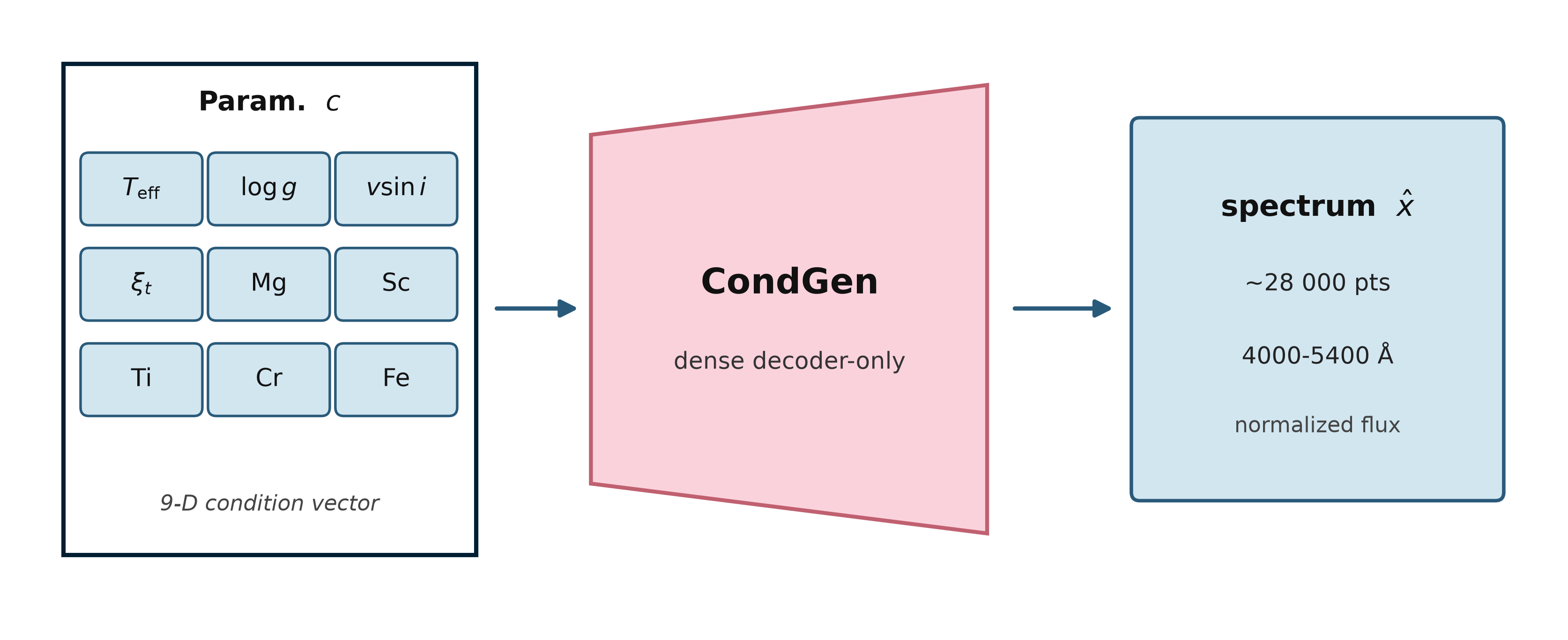 Figure 1. Workflow summarized from the account in Appendix A. Left feedback returns a critique for technical or editorial correction; right feedback routes a revised human decision into a new assignment. Boxes group functions rather than imply that every role ran concurrently.
The flow proceeds through: Authors (Question, existing data and notebooks, scope, milestone approval) → Orchestrator (Translate approved milestones into specialist assignments) → Specialist work and artifact exchange (Python / Curator: numerical work and provenance; Scout / Artist / Editor: references, figures, and manuscript) → Critique and checks (Domain Critic / Auditor; manuscript Reviewer when assigned; Return concerns for correction or identify unresolved evidence) → Authors' decision through the Orchestrator (Accept, revise, retain a limitation, or defer a claim) → Research outputs (Notebooks, evaluation records, figures, and Overleaf manuscript).
2.4. Study basis and workflow evidence
Appendix A presents the workflow as a sequential account of human decisions, specialist assignments, reviews, and research outputs. It is based on a retrospective summary prepared by the Orchestrator and supplied by us. The summary describes project exchanges and handoffs; the underlying conversation logs are not included in the supplied material. The appendix paraphrases that account rather than reconstructing verbatim dialogue.
We distinguish decisions and handoffs reported in the workflow account, manuscript content and figure assets present in the project, and execution details that remain unverified from the supplied material. A reported training launch does not establish completed training, and internal review labels do not constitute independent replication. The available evidence supports an ordered qualitative account, without reliable event-by-event timestamps, complete task counts, token usage, costs, or human time measurements.
The project record identifies the platform and describes the responsibilities assigned to each bot. It does not include the complete setup instructions needed to recreate the team. The descriptions presented here therefore explain how the research tasks were divided and coordinated. They do not establish whether the bots used different underlying models or performed their tasks simultaneously.
2.5. Collaboration illustrated by consequential decisions
Four examples show how assignments, critique, and human decisions affected the research outputs. Their full sequence and supporting context appear in Appendix A; they are selected examples, not a count of all tasks completed.
Evaluation protocol. The Python/Jupyter Specialist and the Spectroscopy Domain Critic identified an inconsistency in the model evaluation: one assessment used preprocessing scalers that differed from those used during training. The account reports an MAE of approximately 0.024 with the mismatched scalers, compared with 0.003681 when the training-matched scalers were used. We accepted the latter evaluation for reporting the model's performance. Although the two evaluations also differed in numerical precision, the available comparison does not establish which changes contributed to the difference in error (Appendix A.3).
Negative-result reporting. The bot team identified the cool-star Mg limitation, and the Critic challenged the interpretation of the diagnostic. We approved retaining the diagnostic and explicitly reporting the limitation. The resulting changes concerned the claim and its presentation; they did not resolve the discrepancy's cause (Appendix A.4).
Model selection. Four short architecture pilots did not displace the dense baseline in the reported comparison. We approved a comparison with caveats about training budgets and test-subset provenance, rather than a general architectural ranking (Appendix A.5).
Manuscript production. The Orchestrator coordinated numerical information from Python, figures from the Artist, references from the Scout, and integration by the Editor, with critique and human review between these steps. Checks corrected presentation and citation problems (Appendix A.6).
2.6. Observed outcomes and limits of measurement
Table 2 summarizes the evidence available for assessing the workflow. The observable contribution is a set of reported corrections, decisions, and coordinated outputs. Neither the number of roles nor the number of selected episodes is a success rate. No human-only or single-agent comparison was conducted in the supplied record, and no complete accounting of time or cost is available. We discuss our retrospective estimate of elapsed project time in Section 7.
2.7. Relation to prior agent workflows and limitations
Previous projects, including Agent Laboratory, ResearchAgent, the Virtual Lab, Coscientist, and SciAgents, have explored how AI agents can support scientific research through different forms of collaboration [18–22]. Our study contributes a practical example from astronomy, showing how a team of specialized bots participated in numerical analysis, scientific review, figure preparation, and manuscript development. Its contribution lies in describing how these activities were connected and how exchanges among the agents and us influenced the research outputs.
The examples presented here illustrate useful scientific and technical contributions from the bots. These include identifying an inconsistent evaluation procedure, detecting the cool-star Mg limitation, and coordinating the preparation of figures and text. Human supervision was an integral part of this approach: we defined the research objectives, reviewed the agents' findings, and made decisions about interpretation and reporting.
The main limitation concerns the completeness of the available documentation. The workflow account was reconstructed from a summary prepared by the Orchestrator after the work, rather than from a complete archive of conversations and execution records. It therefore describes selected contributions and decisions, but does not support a systematic measurement of how often the team succeeded, how much human intervention was required, or how its performance compared with another research arrangement. The time comparison discussed in this paper reflects our retrospective estimate rather than a controlled measurement.
Review by specialist bots provided opportunities to identify errors and question scientific claims. However, agents using similar models or shared information may also make similar mistakes. Their agreement, or an internal review label such as PASS, cannot replace verification of the underlying calculations and evidence. The Mg finding illustrates the value of agent critique, while its unresolved cause shows where further investigation is needed.
Future studies could strengthen this approach by preserving the bot instructions, task assignments, review exchanges, numerical outputs, and human decisions alongside the code and data [23–25]. Such records would make the workflow easier to reproduce and allow a more precise assessment of its reliability, efficiency, and requirements for human supervision.
Table 2. Workflow outcomes and evidential limits. The retrospective account is included in Appendix A; reported decisions and outputs are distinguished from missing execution evidence.
| Aspect | Available evidence | What remains unestablished |
|---|---|---|
| Protocol correction | The workflow account reports rejection of mismatched scalers and retention of the training-matched recipe | Raw before/after evaluations and isolated cause of the discrepancy |
| Negative-result handling | Bots identified the Mg limitation; the authors approved reporting it; the diagnostic figure is present | Root cause and robustness across atmospheric conditions |
| Architecture choice | Four pilot alternatives and a comparison table | Matched training budgets, complete run records, and generalization of the ranking |
| Manuscript coordination | The workflow account describes parameter-to-figure-to-editor handoffs and compile reports from the project | Complete message chronology and artifact-to-run manifest |
| Human oversight | Author decisions on scope, reporting the bots' Mg finding, model choice, and training | Complete intervention count or measured author effort |
| Efficiency and cost | Authors' retrospective time estimate; no complete time or cost logs | Measured labor or runtime savings, cost savings, or superiority over alternatives |
Part B: CondGen scientific case study.
3. Related Work
Part B is the scientific application and case study under the AI-agent workflow of Part A: it builds on our prior generative architectures and stellar databases [7,8] without demoting the astrophysical content. Neural-network surrogates for stellar spectra now span deterministic label-to-flux emulators, conditional generative synthesizers, large-scale foundation and transfer models, and synthetic-to-observed domain adapters. We situate the present CondGen study in that landscape while stating its scope narrowly: abundance-conditioned generation of optical stellar spectra at fixed resolving power \(R\), trained and evaluated entirely in the synthetic domain. Inverse abundance recovery, survey pipeline deployment, and domain adaptation are out of scope for this manuscript.
3.1. Spectral emulators and abundance-aware forward models
The dominant survey paradigm remains the deterministic emulator that maps atmospheric labels, including individual elemental abundances, onto flux, then recovers labels by \(\chi^2\) or related fitting. The Payne [11] established this pattern for high-resolution spectra with many abundance dimensions. Subsequent work improves accuracy, spectral coverage, and survey readiness: TransformerPayne replaces multilayer perceptrons with attention suited to long-range line correlations and improves data efficiency [13]; LRPayne targets low-resolution (\(R \sim 5000\)), WEAVE-like settings with a large abundance vector [12]; data-driven Payne variants (DD-Payne) learn from survey spectra themselves to deliver homogeneous elemental abundances for DESI and LAMOST FGK samples [26,27]; hybrid SLAM–Payne frameworks address early-type stars on LAMOST low-resolution data [28]; and NLTE-aware Payne-style networks prepare chemical diagnostics for 4MOST-scale high-resolution surveys [29]. Scaling studies quantify how emulator error depends on grid size and architecture capacity [30], while next-generation physical-model stacks aim at spectrum synthesis in seconds [31].
These works establish abundance-aware label-to-flux prediction as a relevant baseline. CondGen also implements a deterministic label-to-flux map. Its present use emphasizes forward fidelity to synthetic spectra under five elemental abundance conditions, rather than an implemented inverse-fitting pipeline. This difference in application does not make the network a stochastic sampler or imply a fundamental architectural distinction from deterministic emulators.
3.2. Generative and physics-embedded spectral synthesis
A smaller literature builds neural generators that synthesize spectra from labels (or latents) rather than only emulating them for fitting. Gebran [7] combined an autoencoder with a dense parameter-to-latent map to regenerate Gaia RVS synthetic spectra (approximately 8400–8800 Å) from global stellar parameters including bulk metallicity [M/H]. Gebran & Bentley [8] replaced that two-stage stack with a conditional variational autoencoder (CVAE) over an optical window (approximately 4450–5400 Å), still conditioning on global parameters, including \(T_{\rm eff}\), \(\log g\), \(v_e \sin i\), [M/H], microturbulence, and resolving power \(R\), and explicitly leaving individualized elemental abundances as future work.
Physics-informed generative directions push beyond purely data-driven synthesis: PhysFormer embeds radiative-transfer / flux-conservation structure in the generative mechanism itself [32], while PINN atmosphere models enforce hydrostatic (and related) constraints in a differentiable setting [33]. Score-based diffusion has begun to appear for posterior stellar spectrum sampling in exoplanet contexts through POSTELLAR [34]. Domain-translating GANs for template libraries occupy an adjacent generative niche but target observed realism rather than SYNSPEC fidelity [35].
We extend our earlier spectral-generation work along the abundance axis. We summarize the differences between our previous generative SYNSPEC surrogates and the present CondGen study in Table 3.
The contribution is an extension of our existing spectral-generation program to individual abundances at fixed resolving power, used here as a research-workflow case study. No priority claim for neural spectral generation is made. The model is data-driven; it does not implement the physics-embedded mechanism of PhysFormer or the diffusion sampling of POSTELLAR.
3.3. Foundation and transfer models
Self-supervised and foundation-style spectral models grew rapidly in 2023–2026. Transformer foundation models for stars support multi-survey representation learning, parameter inference, and spectrum generation / inpainting [36]. SpectraFM pretrains transformers on large synthetic APOGEE-like grids and transfers toward observed spectra and few-shot abundances [37]. SpecCLIP aligns and translates spectroscopic measurements across instruments (e.g. LAMOST LRS to and from Gaia XP) with abundance-relevant downstream hooks [38]; LoRA fine-tuning adapts such models across surveys with modest compute [39]. OmniSpectra targets native-resolution multi-survey unification [40]. Cross-modal galaxy image–spectrum models such as AstroCLIP illustrate related architectural ideas outside the stellar CondGen claim [41].
We cite this literature only as landscape. The present CondGen is not a foundation model, not contrastive pretraining at SpecCLIP/SpectraFM scale, and not a cross-survey transfer product.
Table 3. Contrast among our generative spectra surrogates and the present CondGen study.
| Axis | Gebran (2024) AE [7] | Gebran & Bentley (2025) CVAE [8] | This work (CondGen) |
|---|---|---|---|
| Wavelength | Gaia RVS ∼8400–8800 Å | Optical ∼4450–5400 Å | Optical ∼4000–5400 Å |
| Conditioning | Global [M/H] (+ Teff, log g, v sin i, ξt) | Global [M/H] (+ Teff, log g, v sin i, ξt); R free | Elemental abundances Mg, Sc, Ti, Cr, Fe (+ atmospheric labels); R fixed |
| Generative form | Autoencoder + dense parameter→latent map | Conditional VAE (CVAE) | Deterministic dense label-to-spectrum map; no latent sampling |
| Domain / task | Synthetic SYNSPEC regeneration | Synthetic SYNSPEC regeneration | Synthetic-only forward fidelity; inverse recovery shelved |
3.4. Domain adaptation: deliberate out of scope
Unsupervised and GAN-based bridges between synthetic and observed spectra are mature: Cycle-StarNet remains a canonical cycle domain-adaptation approach between theoretical and survey spectra [42], and SOST constructs generative-adversarial template libraries that translate toward observed LAMOST-like realism [35]. Those goals are scientifically important but orthogonal to a synthetic-only CondGen fidelity study. We therefore cite them once as a deliberate scope boundary.
3.5. Positioning of this work
In summary, abundance-aware deterministic emulators (Payne lineage) and survey UQ tools such as conditional invertible networks [43,44] define the fitting/inference frontier; foundation models define the transfer frontier; Cycle-StarNet/SOST define the domain-adaptation frontier; PhysFormer and POSTELLAR define physics-embedded and diffusion generative frontiers. Against that backdrop, this paper's contribution is tightly scoped: an abundance-conditioned CondGen for optical stellar spectra (Mg, Sc, Ti, Cr, Fe and related labels), trained in the synthetic domain at fixed \(R\), with forward fidelity as the primary scientific product of the case study. It extends Gebran & Bentley [8] from global [M/H] to elemental abundance axes, and it is architecturally and wavelength-distinct from the Gaia RVS autoencoder generator of Gebran [7]. Inverse abundance recovery from CondGen spectra is shelved for a separate study and is not centered here.
4. Database
The CondGen case study uses a database of synthetic spectra representative of A-, F-, G-, and K-type stars. The calculations follow the atmosphere and spectral-synthesis framework used in our previous studies [7,8]. In this framework, ATLAS9 [45] provides the stellar model atmospheres, describing how temperature, pressure, and density vary with depth for a specified effective temperature, surface gravity, and chemical composition. These one-dimensional atmospheres adopt a plane-parallel geometry, hydrostatic equilibrium, and local thermodynamic equilibrium (LTE), in which the local temperature and density determine the atomic level populations. Line blanketing accounts for the combined influence of numerous absorption lines on the atmospheric structure and the redistribution of radiation. The framework also includes convective energy transport in cooler atmospheres, as described in our earlier work.
The resulting atmospheric structures are supplied to SYNSPEC [46], which solves the radiative-transfer equation to calculate the emergent spectrum over the selected wavelength interval. Continuum and spectral-line opacities determine the wavelength-dependent flux, allowing the effects of the adopted elemental abundances to be represented in the synthetic spectra. These synthetic spectra provide the reference outputs used to train and evaluate CondGen; no observed spectra enter training or the primary fidelity evaluation.
Each training/evaluation spectrum is the SYNSPEC continuum-normalized flux vector. CondGen learns and is scored in that normalized flux space, not in absolute flux or magnitudes. We do not apply an additional empirical continuum re-fit at train or test time.
The database is structured in the same way we did in [7,8] and the bot has reading access to it (∼45 GB on disk). The optical window covers 4000–5400 Å at \(\Delta\lambda = 0.05\) Å (\(N_\lambda = 28\,000\) wavelength points) with a resolving power \(R \simeq 50\,000\). The wavelength abscissa is constructed as
$$\lambda_i = 4000 + i\,\Delta\lambda, \qquad i = 0, \ldots, N_\lambda - 1,$$
equivalently, so the last sampled wavelength is 5399.95 Å. Each continuum-normalized flux vector is paired with classical atmospheric parameters and five elemental abundances. The per-spectrum dump tuple is laid out as
- index 0: continuum-normalized SYNSPEC flux (length \(N_\lambda\));
- indices 1–5: \(T_{\rm eff}\) (K), \(\log g\) (dex), \(v_e \sin i\) (km s⁻¹), \(\xi_t\) (km s⁻¹), and resolving power \(R\) (database metadata; fixed at \(R = 50\,000\));
- index 6: [Mg/H];
- indices 7–10: [Sc/H], [Ti/H], [Cr/H], and [Fe/H].
The CondGen conditioning vector is the standardized 9-D label
$$c = [T_{\rm eff}, \log g, v_e \sin i, \xi_t, {\rm Mg}, {\rm Sc}, {\rm Ti}, {\rm Cr}, {\rm Fe}],$$
i.e. classical atmospheric parameters together with five elemental abundances [Mg/H], [Sc/H], [Ti/H], [Cr/H], and [Fe/H]. Resolving power \(R = 50\,000\) is a fixed database property and is not an input channel of \(c\). Coverage logs for the Abundance CondGen campaign place \(T_{\rm eff}\) in [4000, 10000] K, \(\log g\) in [2.00, 5.00] dex, \(v \sin i\) in [0, 250] km s⁻¹, and microturbulence \(\xi_t\) in [0.5, 3] km s⁻¹, with each of [Mg/H], [Sc/H], [Ti/H], [Cr/H], and [Fe/H] spanning [−1.50, 1.50] dex.
The database contains exactly \(N = 216\,651\) spectra. Wavelength sampling and resolving power are fixed; the varying atmospheric parameters and abundances are described in the project as randomly sampled within the stated ranges.
Using this database, the bots have freezed a stratified train/validation/test partition of the full database (\(N = 216\,651\)) at 80%/10%/10% with a constant seed for reproducibility purposes. We therefore have
$$n_{\rm train} = 173\,325, \quad n_{\rm val} = 21\,669, \quad n_{\rm test} = 21\,657$$
spectra. The supplied interaction summary does not include the seed value, stratification definition, or split manifest. Those execution records are needed to reproduce the reported partition exactly.
5. Conditional Generator
The bot team developed the numerical implementation within the delegated workflow described in Section 2, drawing on our previous papers and the notebooks we provided. These materials supplied the scientific background and an implementation starting point from which the bots proposed modeling choices and planned the calculations. The Orchestrator coordinated this work, the Python/Jupyter Specialist implemented and ran the numerical tasks, and the Spectroscopy Domain Critic reviewed their outputs. We set the scientific scope, specified nine inputs from the outset, and approved the proposed training and evaluation milestones.
5.1. Architecture
CondGen is a dense decoder-only network that maps the standardized 9-D conditioning vector
$$c = [T_{\rm eff}, \log g, v_e \sin i, \xi_t, {\rm Mg}, {\rm Sc}, {\rm Ti}, {\rm Cr}, {\rm Fe}]$$
to a continuum-normalized spectrum \(\hat{x} \in \mathbb{R}^{N_\lambda}\), with \(N_\lambda = 28\,000\). At inference, CondGen produces a single predicted spectrum for each supplied input vector, without stochastic latent sampling, and therefore functions as a deterministic spectral surrogate. Building on their examination of the earlier methods and notebooks, the bot team adopted the dense decoder-only architecture in place of a CVAE formulation to avoid posterior collapse. The schematic is shown in Figure 2.
In practice the decoder is a seven-stage fully connected stack that widens monotonically from the label vector to the spectrum. After the input layer, six hidden dense layers use widths 256, 512, 1024, 2048, 4096, and 8192 units, each with GELU activations and batch normalization. Dropout with rate 0.1 is applied after the 2048-, 4096-, and 8192-unit blocks. A final dense layer with 28 000 units and a sigmoid activation produces the continuum-normalized flux vector. There are no convolutional or recurrent layers and no stochastic latent sampling at inference: the forward map is a deterministic MLP. The reported 9-D build comprises 274 182 496 parameters in total. We do not claim that this capacity is minimal. To assess alternatives, the bot team carried out the ArchSearch pilots described in Section 6.4, comparing the dense baseline with a wider MLP, a FiLM residual network, a multiscale Conv1D network, and wavelength attention under a fixed assessment protocol. The Python/Jupyter Specialist performed the comparisons and the Critic reviewed the findings. The reported pilot results supported retaining the baseline, a decision we approved; they do not establish a general ranking of these architectures.
The bots used our previous spectral-generation studies [7,8] as methodological references when developing the abundance-conditioned CondGen implementation. The 2024 model is a two-stage autoencoder plus dense parameter-to-latent map aimed at Gaia RVS wavelengths with global [M/H]. The 2025 CVAE generates optical SYNSPEC spectra conditioned on \(T_{\rm eff}\), \(\log g\), \(v_e \sin i\), [M/H], microturbulence, and resolving power \(R\). The present Methods fix \(R\) and replace bulk metallicity with elemental abundance axes (Mg, Sc, Ti, Cr, Fe), so comparisons to those priors should emphasize conditioning and wavelength/domain choices rather than recycled residual figures from 2025. Earlier AFGK and A/Am parameter-estimation work, including PCA inversion [9], regularized sliced inverse regression [47], and the deep-learning label trilogy on synthetic then observed AFGK spectra [10,48,49], motivates the optical AFGK database setting and the focus on abundance-sensitive line regions, but those papers are label-inference studies rather than CondGen generators. When describing the forward task, Payne-style networks also implement labels to flux maps with individual abundances [11–13], including NLTE and data-driven survey variants [26,29]; those systems are typically paired with \(\chi^2\) or survey fitting, whereas we train a conditional generative CondGen and score synthetic reconstruction fidelity. Emulator scaling results [30] inform capacity/grid-size discussion only; we do not import their published error numbers as ours. We do not embed RTE residuals or PINN atmosphere constraints in the CondGen loss [32,33], nor do we train score-based diffusion spectrum samplers [34]; such extensions are future work.
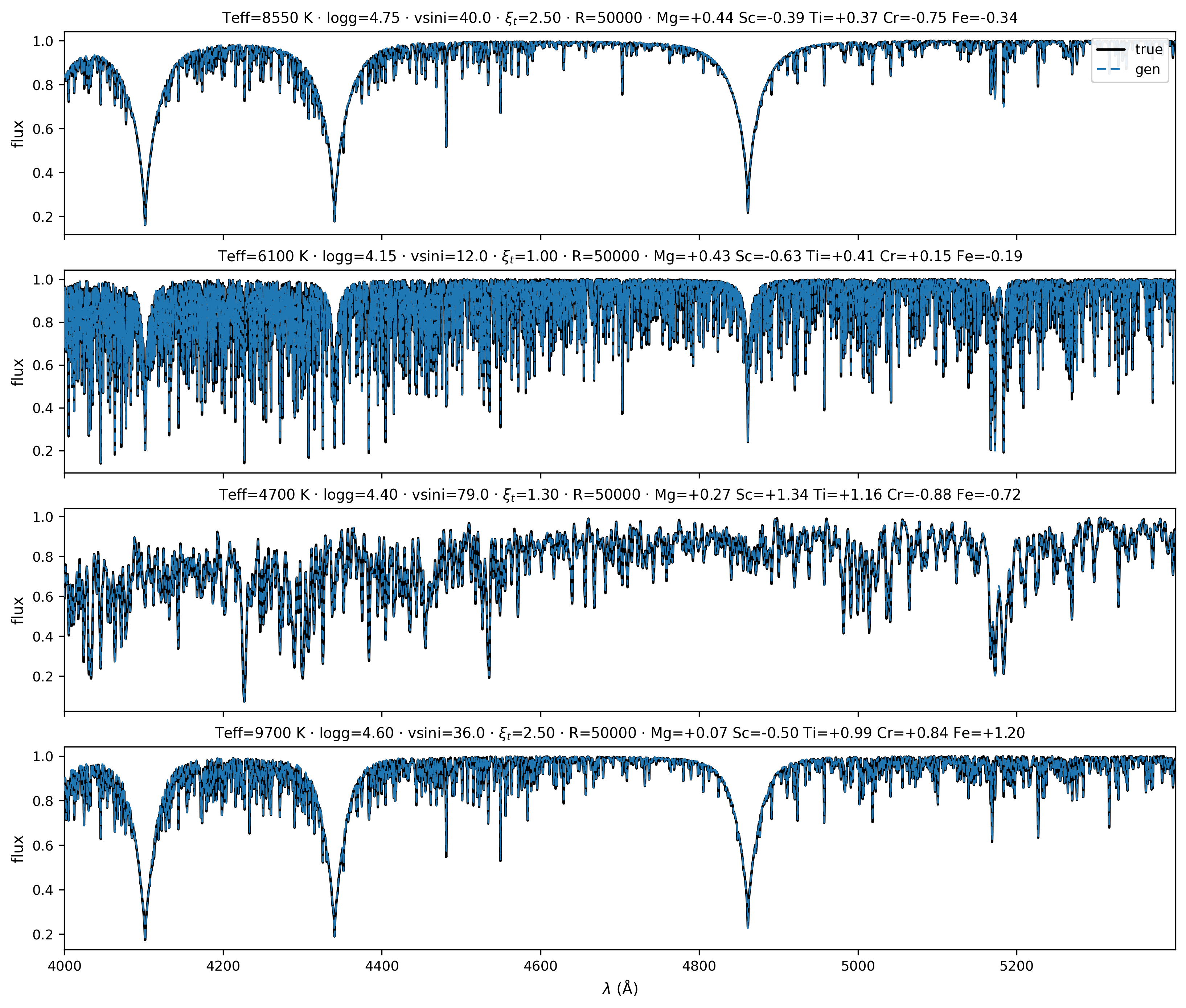 Figure 2. Schematic of the 9-D
 CondGen forward model. A 9-element conditioning vector \(c = [T_{\rm eff}, \log g, v_e \sin i, \xi_t, {\rm Mg}, {\rm Sc}, {\rm Ti}, {\rm Cr}, {\rm Fe}]\) is mapped by a dense decoder-only network to a normalized spectrum \(\hat{x}\) over 4000–5400 Å (\(N_\lambda = 28\,000\)). Resolving power \(R = 50\,000\) is a fixed database property, not an input channel.
Using the supplied notebooks as a starting point, the Python/Jupyter Specialist implemented the training calculations coordinated by the Orchestrator. The documented training recipe combines mean squared error (MSE) and mean absolute error (MAE):
$$\mathcal{L} = 0.8\,{\rm MSE} + 0.2\,{\rm MAE},$$
monitored by validation MAE, with batch size 512 and up to 150 epochs.
6. Scientific case-study results
6.1. Forward-generation metrics and provenance
The bot team used our earlier papers and the supplied notebooks to plan the forward-generation assessments reported in this section. Within the workflow described in Part A, the Orchestrator coordinated the evaluation tasks, the Python/Jupyter Specialist performed the calculations, and the Spectroscopy Domain Critic examined the resulting diagnostics and their interpretation. The following distinctions explain how these activities relate to our published work and to the nine-input model.
- Published background. Our 2024 and 2025 studies [7,8] establish the scientific lineage summarized in Table 3. The bots drew on these studies for methodological context when developing the evaluation approach, while the supplied notebooks provided a starting point for its numerical implementation. The evaluation scores reported below come from the present project's assessments, not from those publications.
- Earlier project assessments. The diagnostic files retained in this project (Figures 3–10) and the recorded architecture scores (Table 4) are discussed in the Orchestrator's retrospective account as material from the baseline assessment and architecture pilot. They illustrate numerical evaluation, figure preparation, critique, and model-selection decisions within the AI-team case study. One narrative source describes these activities, but this does not establish that every output came from a single evaluation run.
- Nine-input model. Figure 2 describes the design specified from the outset: four atmospheric parameters and five abundances, with resolving power fixed outside the input vector. The numerical results below are identified by their recorded assessment context, distinguishing the baseline diagnostics from the 256-spectrum architecture pilot.
The Python/Jupyter Specialist and the Critic identified an assessment that used scalers inconsistent with training. Their diagnosis led to the use of the training-matched preprocessing protocol, and we accepted the resulting baseline MAE of 0.003681 for reporting. This episode connects the numerical result to the bots' checking and correction process, as described in Appendix A.3.
The workflow account supports this distinction between published background, model design, and reported project assessments. It does not replace a per-output record of the notebook, checkpoint, scaler, sample indices, and execution command. Exact run attribution and numerical reproduction remain to be established; the manuscript does not claim that all displayed outputs have been independently verified.
Correlation and \(R^2\) values reported for individual spectra or selected subsets apply to those samples and should not be interpreted as full-test scores. Evaluation reports should specify how each metric is averaged and generate summary figures from the same archived test predictions.
These are synthetic forward-reconstruction diagnostics. They do not measure inverse abundance precision, agreement with observed spectra, or the efficiency of the AI-agent workflow. Numerical status and workflow outcomes are assessed separately (Table 2).
6.2. Project assessment diagnostics and bot autonomy
Figures 3–5 illustrate how specialist bots developed an assigned evaluation task into numerical results, visual diagnostics, and manuscript material. Drawing on the supplied papers and notebooks, the Python/Jupyter Specialist carried out the reconstruction calculations and passed numerical outputs and stellar-parameter information to the Figure Artist. The Artist prepared the diagnostic panels, and the LATEX Editor incorporated them into the manuscript. The Orchestrator coordinated these handoffs, while the Spectroscopy Domain Critic challenged scientific interpretations and presentation choices, prompting revisions through exchanges among the specialists (Appendix A.6).
The bots exercised autonomy within their assigned responsibilities: numerical execution, figure preparation, and technical revisions were handled through the coordinated specialist workflow. Outputs from one bot became inputs for another, allowing the team to advance connected research tasks and respond to critique. We defined the scientific scope, approved milestones, and reviewed the interpretation and reporting. This division of responsibilities illustrates how bot initiative and collaboration operated within human supervision.
The Orchestrator's account associates these figures with the baseline assessment. It describes the collaboration but does not provide a separate execution and review record for each panel. These figures illustrate the reported baseline diagnostics and their role in the bot-led assessment workflow. Figure 3 shows representative SYNSPEC/true (black solid) and CondGen-generated (blue dashed) overlays. The Python-Artist handoff connected calculated spectra to labeled visual comparisons, making agreement and local mismatches available for scientific inspection. This illustrates how one bot's numerical work supported another bot's preparation of a research output.
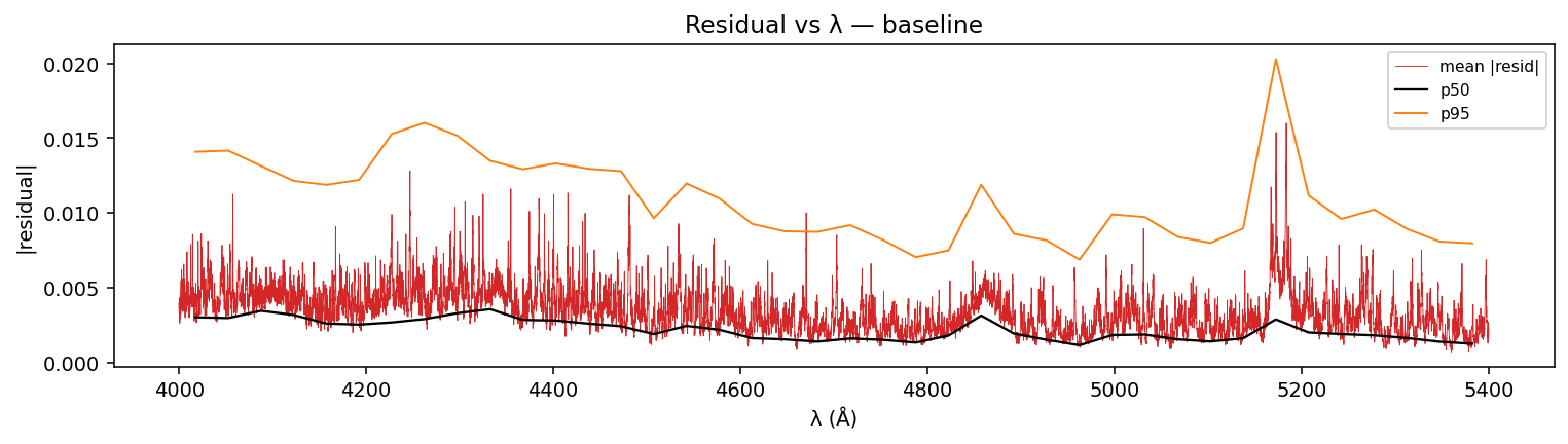 Figure 3. Diagnostic from the project's baseline assessment. Representative SYNSPEC/true (black solid) versus
 CondGen-generated (blue dashed) spectrum overlays. Panel titles list full stellar parameters (\(T_{\rm eff}, \log g, v_e \sin i, \xi_t, R = 50\,000\), Mg, Sc, Ti, Cr, and Fe abundance).
Figure 4 shows selected best-case examples (SYNSPEC/true black solid; CondGen orange dashed). Here, numerical assessment and figure preparation are connected through selection by MAE, illustrating how the bots translated computed results into examples for the manuscript. These selected reconstructions demonstrate close agreement in particular cases; they do not estimate average performance across the test set.
The Python/Jupyter Specialist computed the differences between generated and reference spectra, and the Figure Artist plotted their absolute values against wavelength in Figure 5. The purpose of this bot-produced diagnostic was to examine where reconstruction errors are concentrated across the spectrum. The plot shows the mean absolute residual, the median (p50), and the 95th percentile (p95). Errors are generally larger in the 4000-4500 Å region and lower across much of 4600-4800 Å, with a pronounced local enhancement near 5170 Å. The contrast between larger deviations in regions containing strong or crowded absorption features and smaller deviations in quieter intervals shows that reconstruction quality varies with spectral structure. The separation between the median and the 95th percentile also highlights the spread in residual magnitudes, with larger errors extending beyond the typical level. This diagnostic therefore gave the bot team a way to locate regions requiring closer inspection and supplied the Critic with material for assessing the model's limitations, complementing the selected examples of close agreement.
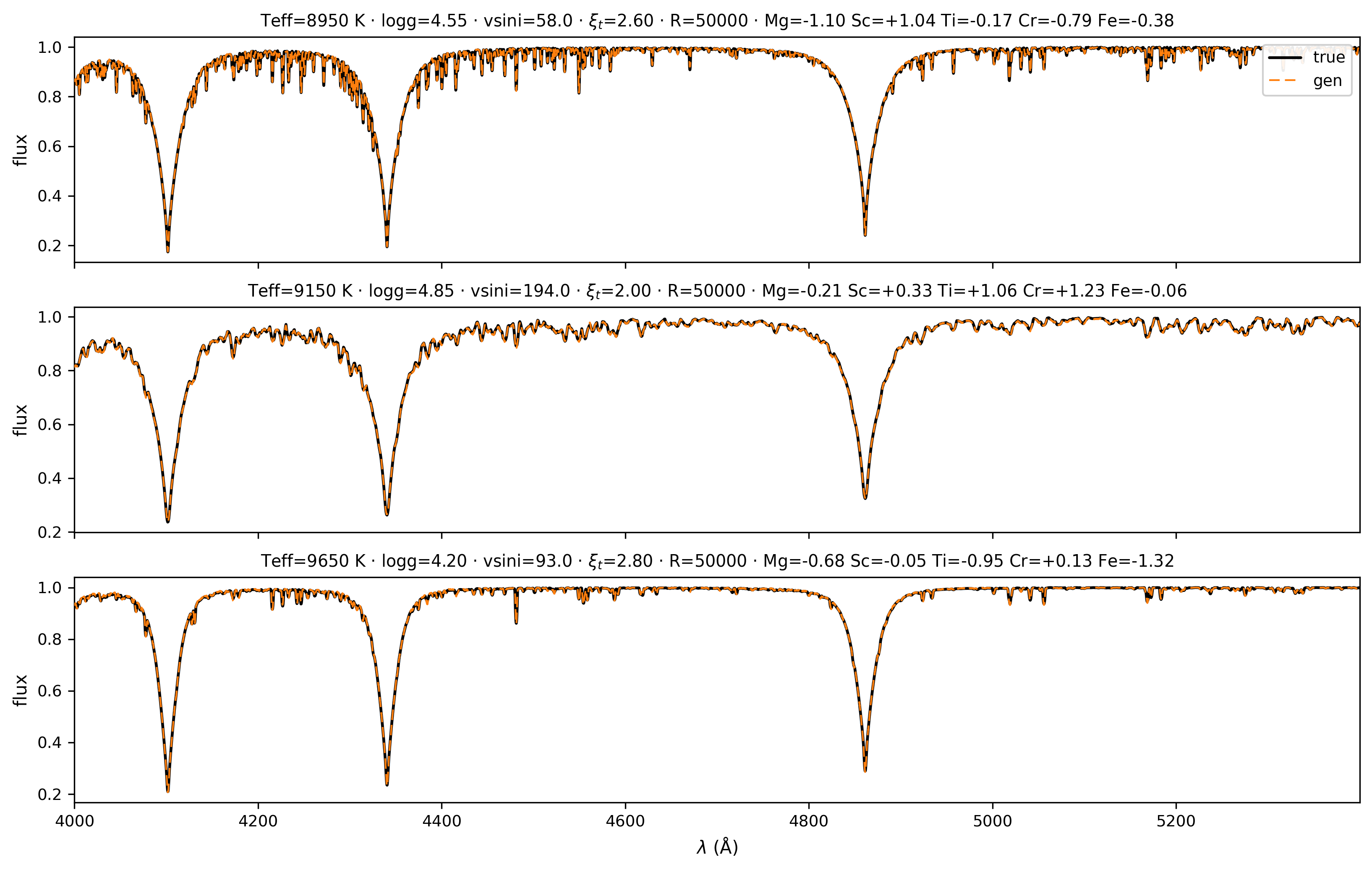 Figure 4. Diagnostic from the project's baseline assessment. Best-case baseline reconstructions (qualitative panel selection by MAE). SYNSPEC/true (black solid);
 CondGen generated (orange dashed). Panel titles show full stellar parameters (\(T_{\rm eff}, \log g, v_e \sin i, \xi_t, R = 50\,000\), Mg, Sc, Ti, Cr, and Fe abundance).
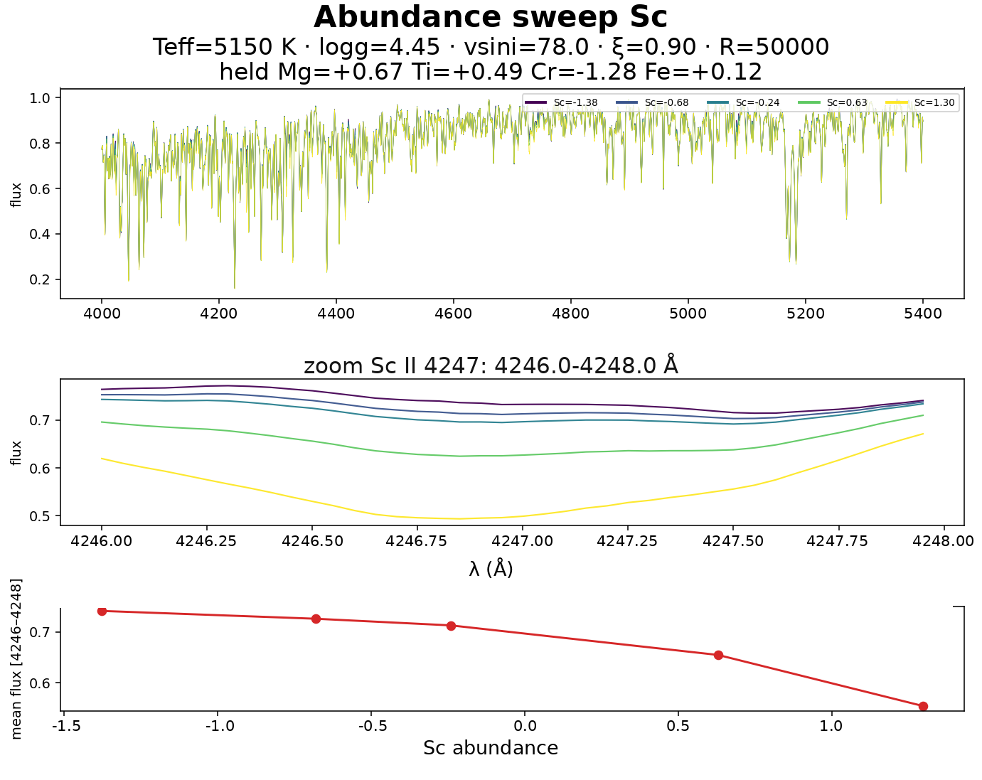 Figure 5. Diagnostic from the project's baseline assessment. Absolute residuals \(|\hat{x} - x|\) between
 CondGen-generated and SYNSPEC spectra as a function of wavelength. The curves show the mean absolute residual (red), median (p50; black), and 95th percentile (p95; orange).
6.3. Abundance sweeps (Sc, Ti, Cr, Fe) and cool-star Mg-line response
The bot team used one-element abundance sweeps to examine how CondGen responds when the chemical composition changes. The Python/Jupyter Specialist varied one abundance while holding the atmospheric parameters and other abundances fixed, and the Figure Artist presented the resulting spectra and line diagnostics. This controlled calculation allowed the Critic to examine whether increasing an abundance produced a consistent change in the corresponding absorption features, and to identify departures requiring further investigation.
The Orchestrator's account records favorable qualitative assessments of the selected Sc, Ti, and Cr responses and a caveat for Fe. The bot team identified the adverse cool-star Mg response, the Critic flagged the limitation, and we approved retaining it with an explicit explanation (Appendix A.4). The plotted curves show the CondGen abundance response; the qualitative comparison with SYNSPEC is described in the workflow account. The supplied evidence lacks the synthesis commands and source arrays needed to reproduce that comparison.
All five sweeps use the atmospheric anchor \(T_{\rm eff} = 5150\) K, \(\log g = 4.45\), \(v_e \sin i = 78.0\) km s⁻¹, \(\xi_t = 0.90\) km s⁻¹, and \(R = 50\,000\). In each sweep, the four elements that are not varied retain their reference abundances: Mg = +0.67, Sc = −1.38, Ti = +0.49, Cr = −1.28, and Fe = +0.12 in dex [X/H]. Colors run from dark purple at the lowest swept abundance to yellow or yellow-green at the highest.
Each figure presents the diagnostic in three steps: the full generated spectrum, a zoom around a selected absorption feature, and the mean flux in the selected wavelength window as a function of abundance. A decrease in mean normalized flux indicates stronger absorption within that window. The bots could therefore inspect both the changing line profiles and a compact measure of their response. These checks assess qualitative behavior at one atmospheric anchor; they do not establish a numerical accuracy threshold across the full label space.
For Sc (Figure 6), the bots examined the feature around 4247 Å.
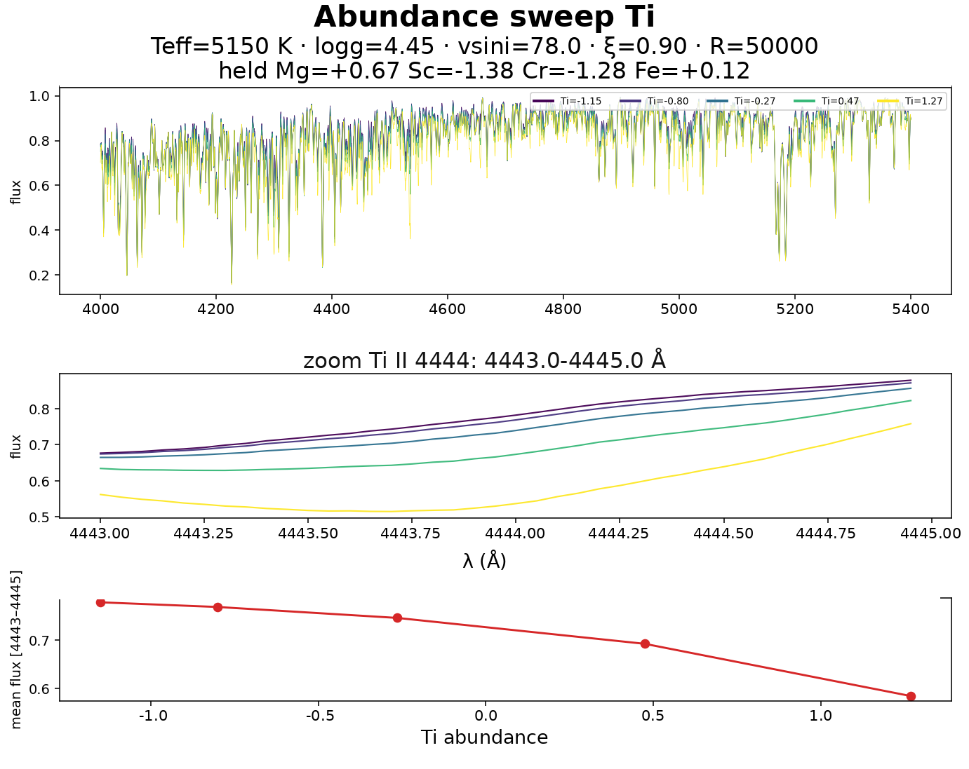 Figure 6. Baseline Sc abundance sweep at the common anchor, showing the Sc II feature around 4247 Å and the decrease in mean flux as abundance rises.
Increasing [Sc/H] lowers the flux in the selected window and deepens the absorption profile, while the mean-flux curve decreases steadily across the sampled abundances. The diagnostic therefore shows a consistent strengthening of the selected feature as Sc abundance increases, supporting the Critic's favorable qualitative assessment at this atmospheric anchor.
For Ti (Figure 7), the bots plotted the response around 4444 Å to test the effect of changing [Ti/H].
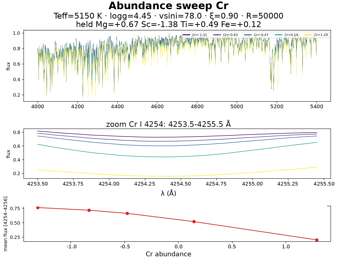 Figure 7. Baseline Ti abundance sweep at the common anchor, showing the Ti II region around 4444 Å and its decreasing mean-flux response.
The higher-abundance curves show deeper absorption, and the mean flux decreases consistently as Ti abundance rises. This output gave the Critic a second example of an orderly abundance response, supporting the reported qualitative acceptance of the Ti diagnostic.
For Cr (Figure 8), the bots examined the feature around 4254 Å.
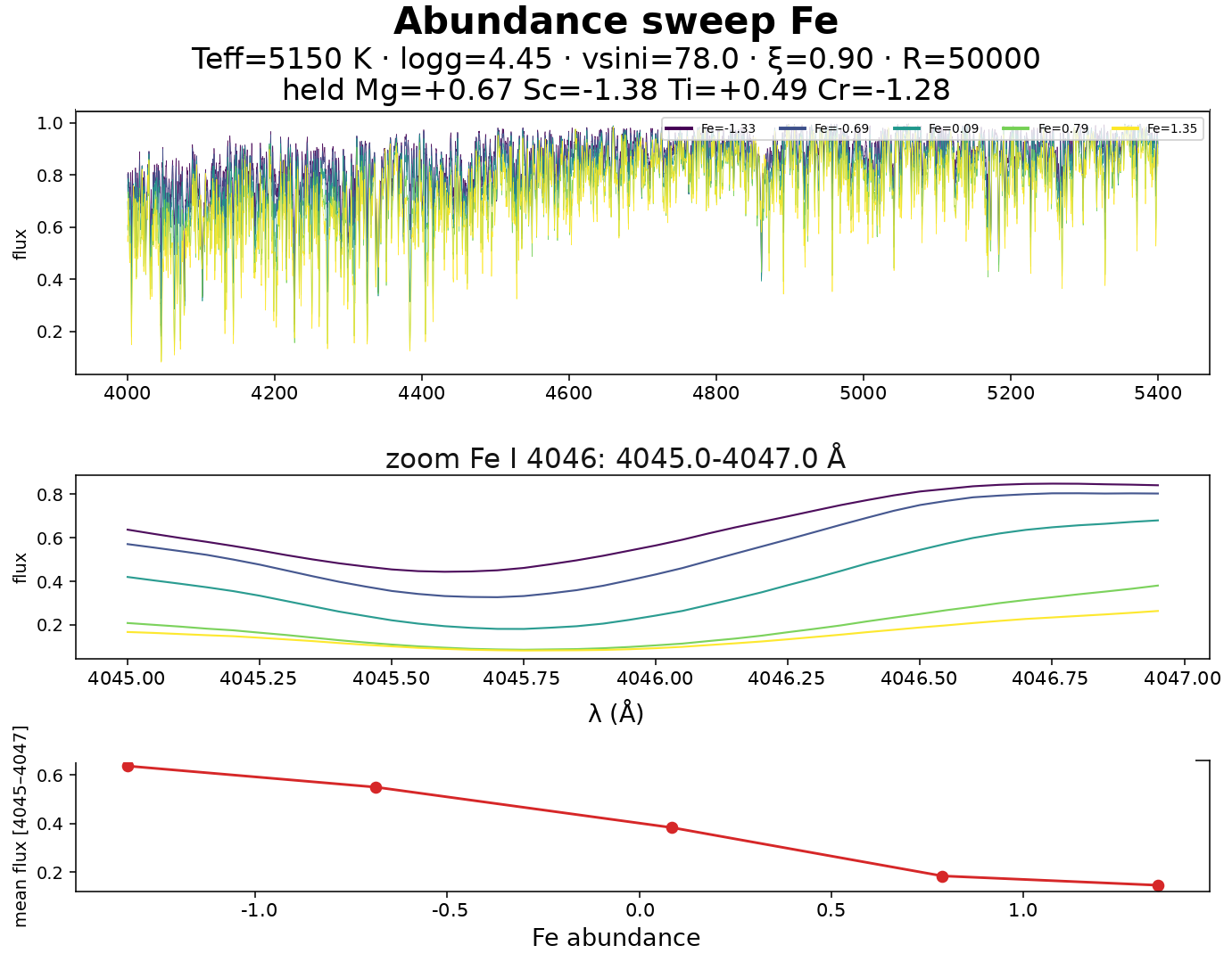 Figure 8. Baseline Cr abundance sweep at the common anchor, showing the Cr I feature around 4254 Å and its decreasing mean-flux response.
The profiles become progressively deeper as [Cr/H] increases, with a corresponding decline in the mean flux. The highest-abundance curve shows the strongest absorption in the displayed sequence. This diagnostic completes the three elemental responses for which the Critic reported favorable qualitative behavior, linking the numerical sweep to an explicit scientific assessment.
For Fe (Figure 9), the bots inspected the feature around 4046 Å.
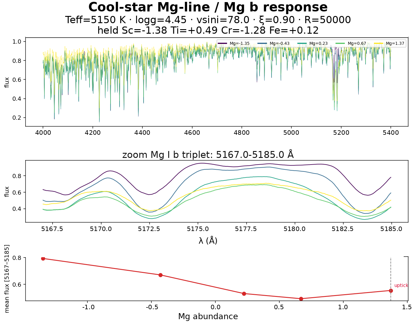 Figure 9. Baseline Fe abundance sweep at the common anchor. The mean-flux response around the Fe I 4046 Å feature flattens toward the highest abundances.
Absorption strengthens as [Fe/H] rises, but the decrease in mean flux becomes smaller between the two highest sampled abundances. This flattening makes the weaker response at the upper end visible. The Critic retained a caveat about high-abundance softening relative to the reference response; the cause is not established by this plot.
For Mg (Figure 10), the bots examined the Mg b region over approximately 5167–5185 Å.
Absorption initially strengthens and the mean flux falls as [Mg/H] rises. At approximately +1.37 dex, however, the mean flux rises relative to the +0.67 dex case and the profiles become shallower. The bot-produced diagnostic therefore reveals a reversal of the earlier trend. The team identified this non-monotonic behavior, and the Critic flagged it as a limitation of the model's cool-star abundance response.
The Mg diagnostic focuses on strong Mg lines, especially Mg b, in cool stars. Mg at the hot anchor was examined only as an internal check and is not shown here.
The cool-star Mg discrepancy identified by the bot team in the project assessment is an empirical limitation. Saturation, blending, training coverage, and model capacity are possible explanations, but the displayed sweeps do not isolate a cause. A dedicated diagnostic study would be required to distinguish them. The sweeps describe behavior at selected atmospheric conditions and do not establish its extent across the full parameter space.
6.4. Architecture comparison (short pilot)
The bot team carried out a short architecture comparison to test whether a different network design could improve spectral reconstruction. The Python/Jupyter Specialist performed the numerical comparisons, the Critic assessed the reported outcomes, and the Orchestrator coordinated the work and communicated the findings. This gave the team a basis for model selection within the project, with us reviewing and approving the resulting choice (Appendix A.5). The bots compared the dense baseline with four alternatives, each testing a different modeling idea:
- Wider MLP: a larger fully connected decoder, used to test whether additional network capacity improved the mapping from stellar labels to spectra.
- Wavelength attention: a decoder using attention across wavelengths, used to test whether this mechanism improved the representation of spectral features.
- Multi-scale Conv1D: a decoder using one-dimensional convolutional filters of different sizes to capture local line structure and broader spectral patterns.
- FiLM residual: a residual network in which the conditioning labels modify intermediate features through feature-wise linear modulation (FiLM), testing another way of incorporating stellar parameters and abundances.
The bots used a common spectral database and fixed data splits, and the project record reports evaluation of all five architectures on a subset of 256 spectra from the test partition. This was a short model-selection exercise, intended to compare the configurations tested for this project. The supplied account does not include complete training and evaluation records for every run, so the results support the pilot decision without establishing a definitive ranking of the architectures.
The bots' comparison identified the dense baseline as the best-performing configuration in this pilot (Table 4). Its MAE of 0.003655 and RMSE of 0.006701 were the lowest recorded values, and its correlation and \(R^2\) were the highest. Wavelength attention was the closest alternative, with an MAE of 0.009588, while the FiLM residual configuration produced the largest errors. The wider MLP and multi-scale Conv1D also failed to improve on the baseline in these runs. These numerical findings supported retaining the baseline, a choice we approved. The unsuccessful alternatives remain in the table so that the basis for that decision is visible.
 Figure 10. Baseline cool-star Mg abundance sweep. The mean-flux rise between approximately +0.67 and +1.37 dex reveals the non-monotonic Mg b response identified by the bots.
Table 4. Architecture comparison on the reported 256-spectrum subset. Scores document the bot team's exploratory evaluation of the tested configurations and the decision to retain the dense baseline.
| Architecture | MAE | RMSE | corr | \(R^2\) |
|---|---|---|---|---|
| Baseline in the pilot | 0.003655 | 0.006701 | 0.9991 | 0.9982 |
| Wavelength attention | 0.009588 | 0.015620 | 0.9951 | 0.9903 |
| Wider MLP | 0.011624 | 0.020060 | 0.9920 | 0.9839 |
| Multi-scale Conv1D | 0.012988 | 0.022033 | 0.9914 | 0.9806 |
| FiLM residual | 0.018974 | 0.052349 | 0.9460 | 0.8905 |
7. Discussion
The principal result of this case study is a documented pattern of delegated work, critique, and human decision-making. The four episodes connect the role descriptions to consequential actions: rejecting an incompatible evaluation recipe, identifying an adverse Mg response through bot analysis and approving its disclosure through human review, limiting the interpretation of pilot results, and coordinating manuscript artifacts. These outcomes make the AI-team contribution concrete while exposing its dependence on existing scientific infrastructure and human supervision.
7.1. Discussion of the AI role
7.1.1. What collaboration contributed
The reported benefit of specialization was a division of responsibilities and interfaces. Python supplied numerical and parameter information; the Artist and Editor turned those outputs into figures and text; the Critic challenged interpretation; and the Orchestrator routed unresolved decisions to us. The Mg episode is especially informative: the bots identified the limitation, the Critic challenged the interpretation, and we approved reporting the adverse result explicitly. Collaboration therefore changed what was claimed while preserving the diagnostic that exposed the problem. The scaler episode similarly shows why evaluation artifacts must be checked against training provenance before numbers enter the paper.
Human input was substantive. We set the problem, supplied the data and notebooks, specified the nine-input design from the outset, approved training, and set the manuscript focus on the AI-team contribution. Describing that involvement only as light final approval would understate the decisions summarized in Appendix A. The case demonstrates how researchers working together can coordinate specialized agents across connected tasks.
A practical benefit we observed was the short turnaround. We estimate that a comparable sequence of implementation, diagnostic review, figure preparation, and manuscript drafting would ordinarily span approximately one academic semester for a professor supervising a team of researchers or students. In this project, the corresponding work was brought together in less than a week through iterative human prompting, interaction with the Orchestrator, and exchanges among specialist bots. This experience illustrates the potential of coordinated AI assistance to shorten the interval between research tasks while we direct the study and review its outputs. The comparison reflects our retrospective estimate of elapsed project time, rather than a controlled measurement of labor savings. It concerns work built on the existing database and notebooks.
7.1.2. What the workflow did not establish
The retrospective source is a participant account rather than a complete execution trace. It cannot establish the frequency of missed errors, the proportion of tasks completed without intervention, or the counterfactual performance of a single agent. Role separation also does not guarantee independent verification.
These limitations suggest concrete improvements to research practice: preserve task identifiers and timestamps; link every numerical claim and figure to code, data, checkpoint, scaler, and evaluation output; retain valid negative results; and record human decisions alongside the agent proposals that prompted them. A prospective study could then compare configurations using task completion, independently checked error rates, human effort, runtime, and cost. Such comparisons were not performed here.
7.2. Discussion of the science case
The CondGen case study represents an important step in our research on stellar spectral generation, extending the conditioning from global metallicity toward individual elemental abundances at fixed resolving power [7,8]. Its nine-input design combines four atmospheric parameters with the abundances of Mg, Sc, Ti, Cr, and Fe, providing a framework for investigating how changes in chemical composition affect generated spectra. As a deterministic forward surrogate, it shares the label-to-flux formulation of established spectral emulators [11–13]. Its value here lies in developing this abundance-conditioned case study through a coordinated AI research workflow.
The reported baseline assessments provide concrete scientific guidance for further development. The bots produced spectral reconstructions, examined the wavelength dependence of their errors, varied individual abundances, and compared alternative architectures. The Sc, Ti, and Cr sweeps showed consistent strengthening of the selected absorption features, while the Fe and Mg diagnostics identified responses that deserve closer investigation. In particular, the cool-star Mg limitation discovered by the bots defines a specific research question: under which conditions does the model cease to reproduce a consistent abundance response, and how can that behavior be improved? These findings turn the case study into a focused program of testable questions, with the scope of the reported assessments specified in Section 6.1.
A more detailed study could build directly on these results by extending the diagnostic sweeps across temperature, surface gravity, and abundance, and by testing how training coverage and model design affect the regions with the largest residuals. Targeted Mg experiments could examine the contributions of strong-line behavior, blending, and the learned spectral mapping. Architecture comparisons with matched training budgets and independent evaluation data would help identify which changes improve reconstruction accuracy. The current work supplies the scientific motivation and initial diagnostics for these investigations, supporting a practical route toward more reliable abundance-conditioned spectral generation.
The project also provides a feasible foundation for sustained research development. The existing spectral database and notebooks can support successive experiments, while the division of work among computation, scientific critique, visualization, and writing provides an organized way to carry those experiments through to interpretation and communication. Under our direction, the Orchestrator could coordinate these follow-up tasks and the specialist bots could implement, assess, and document the resulting improvements. When it identifies a need for additional expertise or capacity, the Orchestrator could create new specialist bots, define their responsibilities, and integrate their contributions into the existing team. The team could thus evolve in response to new research questions and issues raised during analysis or review. This combination of reusable resources, concrete scientific questions, and coordinated AI contributions makes the study a valuable step toward a continuing research program in abundance-conditioned spectral generation.
8. Conclusion
This work demonstrates the practical value of organizing specialized AI bots as a research team under human scientific direction. In the CondGen case study, the bots contributed numerical implementation, spectral diagnostics, architecture comparisons, scientific critique, visualization, and manuscript preparation. Their interactions helped identify an inconsistent evaluation procedure and a limitation in the cool-star Mg response, while we guided the research questions, assessed the interpretations, and approved the reporting. The main contribution is a concrete example of how human judgment and coordinated bot activity can support connected stages of a scientific investigation.
The experience points to an opportunity to increase the pace of research by shortening the cycle between a question, its computational investigation, critical assessment, and the next experiment. Building on our existing database and notebooks, the reported analysis, figure preparation, and manuscript-drafting tasks were brought together in less than a week. This retrospective timing estimate motivates more systematic studies of research efficiency. The potential benefit extends to giving researchers greater capacity to explore alternatives, follow up unexpected findings, and learn from unsuccessful approaches.
The case presented here is a starting point for more complex forms of human-bot collaboration. Future projects could involve larger numbers of specialist bots and several human researchers, each supported by a team of agents. Bots could work independently within defined assignments, while their Orchestrators coordinate the exchange of data, code, and findings across teams. One group could develop models, another examine their statistical robustness, and another attempt to reproduce the results. The human researchers would bring these contributions together, compare interpretations, and set the shared scientific direction. When new questions or gaps in expertise emerge, the Orchestrators could create additional specialist bots and integrate them into the collaboration. This would allow the organization of the research team to evolve with the investigation.
Although this case study was carried out using Grok Bot, the approach is not inherently tied to that platform or to a single AI provider. The principles of task delegation, specialist collaboration, critique, and human supervision can be adapted to other suitable AI systems. Future improvements in AI algorithms, agent-coordination tools, and integration with scientific software could make these teams easier to establish and manage. Such developments could reduce the practical effort required to organize human–bot collaboration and make increasingly complex research projects accessible to a wider range of research groups.
For our case study application, this approach offers a practical route toward broader abundance-response studies, a more detailed investigation of the Mg limitation, and extensions from synthetic to observed stellar spectra. Coordinated bot teams could prepare observational data, investigate differences between simulated and real spectra, implement candidate methods, and evaluate their performance through shared diagnostics and scientific review. These tasks would extend the present case into a more demanding research program while reusing its data, numerical tools, and division of responsibilities.
Realizing this broader vision requires clear task ownership, accessible experiment records, and reproducible checks of the results. Prospective studies should examine how different team sizes and coordination strategies affect reliability, human effort, elapsed time, and cost. The wider opportunity is a research environment in which human insight and bot autonomy reinforce each other: researchers can pursue more questions, learn more quickly from negative results, and move promising ideas toward reproducible evidence. This case study provides a concrete foundation for exploring that future and for accelerating investigation and discovery through collaboration among human researchers and their evolving teams of AI specialists.
Appendix A. Research workflow: a sequential account
This appendix follows the study from the human research brief through numerical work, critique, and manuscript preparation. It is based on the retrospective summary prepared by the Orchestrator and supplied by us; it is not a verbatim conversation transcript. The stages organize the reported work into a readable sequence, while recognizing that some specialist tasks overlapped. We worked collaboratively in directing and reviewing the research; the role names identify the agents' assigned responsibilities.
Appendix A.1. Setting the research brief and assigning responsibilities
We supplied the scientific question, the synthetic spectral database, prior notebooks, and the existing research framework. The project combined two purposes: carrying out an abundance-conditioned spectral-modeling case study and documenting how we could coordinate a team of AI specialists. The manuscript's central contribution was the research workflow, with the astrophysics providing substantive tasks and constraints.
The Orchestrator translated the brief into proposed milestones. We approved or adjusted their scope before specialist work was assigned. The plan connected data preparation, Python/Jupyter execution, scientific checks, figure production, and manuscript assembly. Authorization to assess a model was treated separately from authorization to train it. We also requested visible notebook execution so that numerical work could be inspected. We provided the research direction and remained responsible for scientific decisions and the final manuscript.
Appendix A.2. Inspecting the data and running the training workflow
The Curator and Python/Jupyter Specialist worked with the database and notebooks we supplied to prepare the numerical study. Their tasks connected the stored stellar parameters and abundances to the nine-input design, organized the spectra and data partitions, and maintained the preprocessing information needed for training and assessment. The nine stellar labels were already part of the scientific dataset; the bots' contribution was to identify and use the relevant fields correctly and turn the supplied material into an executable modeling workflow.
The Python/Jupyter Specialist implemented and ran the training calculations. During training, optimization adjusted the network's weights and biases by comparing its generated spectra with the reference spectra. These learned quantities are the model parameters determined through training, distinct from the stellar labels supplied as inputs. Python also supplied the layer dimensions and parameter-count information used by the Artist to explain the architecture. For assessment, the saved model weights had to be paired with the corresponding training scalers and test selection. The Orchestrator coordinated these numerical outputs with the Critic's checks and the Artist's figures, allowing the specialists to build on one another's work.
Appendix A.3. Detecting and correcting the scaler mismatch
The scaler episode illustrates how the bots identified a problem in their own numerical workflow and corrected it. An assessment of the CondGen baseline produced a test MAE of approximately 0.024. The Python/Jupyter Specialist and the Critic checked the evaluation preprocessing against the training setup and identified a mismatch between the scaler files being used. Python corrected the evaluation by using the training-matched scalers; the resulting baseline assessment gave an MAE of 0.003681. The Orchestrator communicated the diagnosis and corrected result to us, and we approved using the training-matched assessment in the manuscript.
The technical detection and correction therefore arose within the bot team: a numerical result prompted criticism, the specialists checked its cause, and the evaluation procedure was revised. Our role was to review the explanation and approve how the result was reported. The mismatched scalers were stored in float64, whereas the training-matched scalers used float32. Because both scaler identity and numerical precision differed, the approximately 6.5-fold change in MAE demonstrates the importance of matching preprocessing to training; it does not show that lower numerical precision is intrinsically more accurate.
Appendix A.4. Reviewing abundance diagnostics
The numerical and figure workflow produced abundance sweeps for comparison with SYNSPEC references. The Critic reviewed their interpretation rather than accepting every plotted trend as physical validation. The account records favorable qualitative assessments of selected Sc, Ti, and Cr diagnostics, a caveat for the softened high-abundance Fe response, and an adverse assessment of the cool-star Mg response.
The bot team identified the Mg limitation in the project diagnostics: at high abundance, the predicted line shallowed or reversed while the reference line continued to deepen. The Critic rejected presenting this response as a clean demonstration of physical fidelity. The Orchestrator communicated the finding to us, and we decided to retain the diagnostic and report the limitation explicitly. It then coordinated that decision with the manuscript and figure workflow, so the adverse result remained visible in Figure 10.
This stage distinguishes the bots' identification and critique of the Mg limitation from our decision about its reporting. The finding arose from the agents' analysis; our role was to approve its inclusion and presentation in the manuscript. It did not establish the physical or numerical cause of the Mg discrepancy. The selected sweeps are qualitative examples of the model response at the atmospheric conditions examined in the project assessment.
Appendix A.5. Comparing alternative architectures
The Python workflow assessed four alternatives to the dense baseline: a wider MLP, wavelength attention, multi-scale Conv1D, and FiLM residual. The Orchestrator reported that none displaced the baseline in the short pilot. We authorized presentation of the comparison with explicit limits and retained the baseline. Section 6.4 reports the scores for the 256-spectrum subset. This was an exploratory comparison used in model selection; it did not constitute an independent final validation of the full parameter space.
The team therefore used the comparison to support a project decision. Complete per-pilot training budgets, stopping criteria, and the exact subset-selection record are unavailable in the supplied evidence, so the result does not establish a general architectural ranking. The retrospective account also reports exclusion of failure panels from the figure set. The poor scores and reported FiLM instability remain disclosed, but the missing panels limit inspection of that failure. These limits belong to the evidence for the decision, rather than being evidence that the baseline is universally preferable.
Appendix A.6. Coordinating figures, references, and manuscript review
The Orchestrator coordinated a manuscript group involving the Editor, Literature Scout, Critic, Artist, and Expert Spectroscopy Reviewer. A separate exchange connected Python and the Artist for numerical and parameter information. Python supplied the values; the Artist used those values to prepare diagrams and diagnostic panels; the Editor inserted the resulting assets into the manuscript. Shared file names and artifact paths connected these steps.
The account describes corrections to overlapping labels and figure borders, as well as a bibliography correction to the LRPayne publication year. The Critic challenged particular claims or displays, while the Expert Reviewer had a distinct manuscript-level role when assigned. We directed the presentation toward the contribution of the AI research team and approved the scientific and editorial choices. Most exchanges were short assignments, acknowledgments, file paths, review labels, or completion reports; the evidence does not describe extended debates between all agents.
The Editor checked figure inclusion and compilation, and the Auditor reported packaging and figure-regeneration checks. These reports support the account of coordinated production but do not replace inspection of the underlying outputs.
Appendix A.7. Applying the nine-input design throughout the workflow
We specified nine inputs from the outset: effective temperature, surface gravity, projected rotational velocity, microturbulence, and the abundances of Mg, Sc, Ti, Cr, and Fe. Resolving power was fixed at \(R = 50\,000\) as a property of the spectral database and was therefore kept outside the input vector. The bots worked within this original scientific specification when preparing the numerical implementation and describing the model.
The Python/Jupyter Specialist supplied the architecture information, including the reported total of 274 182 496 model parameters. The Artist used this information to construct the nine-input architecture diagram, and the Editor incorporated the model description into the manuscript. The Orchestrator coordinated these handoffs so that the numerical work, figure, and written explanation followed the same design. This stage shows how the bots translated a shared research specification into connected computational and communication tasks.
Taken together, these stages show the bots preparing and running numerical work, exchanging results, identifying problems, and revising calculations and their presentation. We provided the scientific direction, reviewed consequential decisions, and remained responsible for the manuscript. The appendix documents selected episodes of this collaborative process from the Orchestrator's retrospective account; complete execution records and measurements of human effort, runtime, and cost would support a more systematic evaluation of its reproducibility and efficiency.
References
- Wang, H.; Fu, T.; Du, Y.; Gao, W.; Huang, K.; Liu, Z.; Chandak, P.; Liu, S.; Van Katwyk, P.; Deac, A.; et al. Scientific discovery in the age of artificial intelligence. Nature 2023, 620, 47–60. https://doi.org/10.1038/s41586-023-06221-2.
- Lawrence, N.D.; Montgomery, J. Accelerating AI for science: open data science for science. Royal Society Open Science 2024, 11. https://doi.org/10.1098/rsos.231130.
- Messeri, L.; Crockett, M.J. Artificial intelligence and illusions of understanding in scientific research. Nature 2024, 627, 49–58. https://doi.org/10.1038/s41586-024-07146-0.
- Li, X.; Wang, S.; Zeng, S.; Wu, Y.; Yang, Y. A survey on LLM-based multi-agent systems: workflow, infrastructure, and challenges. Vicinagearth 2024, 1. https://doi.org/10.1007/s44336-024-00009-2.
- Fluke, C.J.; Jacobs, C. Surveying the reach and maturity of machine learning and artificial intelligence in astronomy. WIREs Data Mining and Knowledge Discovery 2020, 10. arXiv:1912.02934; online Dec 2019, https://doi.org/10.1002/widm.1349.
- Feigelson, E.D.; de Souza, R.S.; Ishida, E.E.O.; Babu, G.J. Twenty-First-Century Statistical and Computational Challenges in Astrophysics. Annual Review of Statistics and Its Application 2021, 8, 493–517. https://doi.org/10.1146/annurev-statistics-042720-112045.
- Gebran, M. Generating Stellar Spectra Using Neural Networks. Astronomy 2024, 3, 1–13. arXiv:2401.13411, https://doi.org/10.3390/astronomy3010001.
- Gebran, M.; Bentley, I. The Use of Conditional Variational Autoencoders in Generating Stellar Spectra. Astronomy 2025, 4, 13. arXiv:2508.17059, https://doi.org/10.3390/astronomy4030013.
- Gebran, M.; Farah, W.; Paletou, F.; Monier, R.; Watson, V. A new method for the inversion of atmospheric parameters of A/Am stars. Astronomy & Astrophysics 2016, 589, A83. https://doi.org/10.1051/0004-6361/201528052.
- Gebran, M.; Paletou, F.; Bentley, I.; Brienza, R.; Connick, K. Deep learning applications for stellar parameter determination: II—application to the observed spectra of AFGK stars. Open Astronomy 2023, 32. arXiv:2210.17470, https://doi.org/10.1515/astro-2022-0209.
- Ting, Y.S.; Conroy, C.; Rix, H.W.; Cargile, P. The Payne: Self-consistent ab initio Fitting of Stellar Spectra. The Astrophysical Journal 2019, 879, 69. arXiv:1804.01530, https://doi.org/10.3847/1538-4357/ab2331.
- Vernekar, N.; Spina, L.; Lucatello, S.; Arcidiacono, C.; Cortese, L.; Simioni, M.; Balestra, A. LRPayne: Stellar parameters and abundances from low-resolution spectra. Astronomy & Astrophysics 2026, 706, A217. arXiv:2511.06546, https://doi.org/10.1051/0004-6361/202556502.
- Rózański, T.; Ting, Y.S.; Jabłońska, M. TransformerPayne: Enhancing Spectral Emulation Accuracy and Data Efficiency by Capturing Long-range Correlations. The Astrophysical Journal 2025, 980, 66. arXiv:2407.05751, https://doi.org/10.3847/1538-4357/ad9b99.
- Nature Editorial. Tools such as ChatGPT threaten transparent science; here are our ground rules for their use. Nature 2023, 613, 612. https://doi.org/10.1038/d41586-023-00191-1.
- Thorp, H.H. ChatGPT is fun, but not an author. Science 2023, 379, 313. https://doi.org/10.1126/science.adg7879.
- COPE Council. Authorship and AI tools. COPE position statement, 2024. https://doi.org/10.24318/cCVRZBms.
- Hosseini, M.; Resnik, D.B.; Holmes, K. The ethics of disclosing the use of artificial intelligence tools in writing scholarly manuscripts. Research Ethics 2023, 19, 449–465. https://doi.org/10.1177/17470161231180449.
- Schmidgall, S.; Su, Y.; Wang, Z.; Sun, X.; Wu, J.; Yu, X.; Liu, J.; Moor, M.; Liu, Z.; Barsoum, E. Agent Laboratory: Using LLM Agents as Research Assistants. In Proceedings of the Findings of the Association for Computational Linguistics: EMNLP 2025, Suzhou, China, 2025; pp. 5977–6043. arXiv:2501.04227, https://doi.org/10.18653/v1/2025.findings-emnlp.320.
- Baek, J.; Jauhar, S.K.; Cucerzan, S.; Hwang, S.J. ResearchAgent: Iterative Research Idea Generation over Scientific Literature with Large Language Models. In Proceedings of the 2025 Conference of the Nations of the Americas Chapter of the Association for Computational Linguistics: Human Language Technologies (Volume 1: Long Papers), Albuquerque, New Mexico, 2025; pp. 6709–6738. arXiv:2404.07738, https://doi.org/10.18653/v1/2025.naacl-long.342.
- Swanson, K.; Wu, W.; Bulaong, N.L.; Pak, J.E.; Zou, J. The Virtual Lab of AI agents designs new SARS-CoV-2 nanobodies. Nature 2025, 646, 716–723. https://doi.org/10.1038/s41586-025-09442-9.
- Boiko, D.A.; MacKnight, R.; Kline, B.; Gomes, G. Autonomous chemical research with large language models. Nature 2023, 624, 570–578. arXiv:2304.05332, https://doi.org/10.1038/s41586-023-06792-0.
- Ghafarollahi, A.; Buehler, M.J. SciAgents: Automating Scientific Discovery Through Bioinspired Multi-Agent Intelligent Graph Reasoning. Advanced Materials 2025, 37, 2413523. arXiv:2409.05556, https://doi.org/10.1002/adma.202413523.
- Pineau, J.; Vincent-Lamarre, P.; Sinha, K.; Larivière, V.; Beygelzimer, A.; d'Alché Buc, F.; Fox, E.; Larochelle, H. Improving Reproducibility in Machine Learning Research (A Report from the NeurIPS 2019 Reproducibility Program). Journal of Machine Learning Research 2021, 22, 1–20. arXiv:2003.12206.
- Kapoor, S.; Narayanan, A. Leakage and the reproducibility crisis in machine-learning-based science. Patterns 2023, 4, 100804. https://doi.org/10.1016/j.patter.2023.100804.
- Wilkinson, M.D.; Dumontier, M.; Aalbersberg, I.J.; Appleton, G.; Axton, M.; Baak, A.; Blomberg, N.; Boiten, J.W.; da Silva Santos, L.B.; Bourne, P.E.; et al. The FAIR Guiding Principles for scientific data management and stewardship. Scientific Data 2016, 3, 160018. https://doi.org/10.1038/sdata.2016.18.
- Zhang, M.; Xiang, M.; Ting, Y.S.; Wang, J.; Li, H.; Zou, H.; Nie, J.; Mou, L.; Wu, T.; Wu, Y.; et al. Determining Stellar Elemental Abundances from DESI Spectra with the Data-driven Payne. The Astrophysical Journal Supplement Series 2024, 273, 19. arXiv:2402.06242, https://doi.org/10.3847/1538-4365/ad51dd.
- Zhang, M.; Xiang, M.; Ting, Y.S.; Amarsi, A.M.; Zhang, H.W.; Shi, J.; Yuan, H.; Li, H.; Wang, J.; Wu, Y.; et al. Homogeneous Stellar Atmospheric Parameters and 22 Elemental Abundances for FGK Stars Derived from LAMOST Low-resolution Spectra with DD-PAYNE. The Astrophysical Journal Supplement Series 2025, 279, 5. arXiv:2506.02763, https://doi.org/10.3847/1538-4365/add016.
- Sun, W. A hybrid SLAM-Payne framework for atmospheric parameter and abundance determination of early-type stars from LAMOST DR9 low-resolution spectra. Astronomy & Astrophysics 2025, 698, A300. arXiv:2505.10310, https://doi.org/10.1051/0004-6361/202554658.
- Storm, N.; Bergemann, M.; Rózański, T.; Ksoll, V.F.; Bensby, T.; Traven, G.; Kordopatis, G.; Church, R.P.; Jian, M.; Sun, W.; et al. Observational Constraints on the Origin of the Elements. X. Combining Non–Local Thermodynamic Equilibrium and Machine Learning for Chemical Diagnostics of 4 Million Stars in the 4MIDABLE-HR Survey. The Astrophysical Journal 2026, 1003, 27. arXiv:2512.15888, https://doi.org/10.3847/1538-4357/ae6108.
- Rózański, T.; Ting, Y.S. Scaling Laws for Emulation of Stellar Spectra. The Open Journal of Astrophysics 2025, 8. arXiv:2503.18617, https://doi.org/10.33232/001c.140607.
- Ting, Y.S.; Kim, E.M. The Payne Zero Project I: Stellar Spectra from Physical Models in Seconds, 2026, [arXiv:astro-ph.SR/2607.24141]. arXiv preprint.
- Wang, S.; Zhang, M.; Bu, Y.; Mou, C. PhysFormer: A Physics-Embedded Generative Model for Physically Self-Consistent Spectral Synthesis, 2026, [arXiv:astro-ph.IM/2603.01459]. https://doi.org/10.48550/arXiv.2603.01459.
- Li, J.; Jian, M.; Ting, Y.S.; Green, G.M. Differentiable Stellar Atmospheres with Physics-Informed Neural Networks, 2025, [arXiv:astro-ph.SR/2507.06357]. ICML 2025 ML4Astro; arXiv preprint.
- Doshi, D.; Cowan, N.B.; Hezaveh, Y.; Barco, G.M.; Artigau, É. POSTELLAR: Posterior Stellar Spectrum Sampling—An Alternative to Approximate Stellar Spectra for Exoplanetary Analysis. The Astrophysical Journal 2026, 1009, 35. arXiv:2609.05599, https://doi.org/10.3847/1538-4357/ae9949.
- Cai, J.; Yan, Z.; Yang, H.; Chen, X.; Zheng, A.; Hao, J.; Zhao, X.; Xun, Y. Stellar spectral template library construction based on generative adversarial networks. Astronomy & Astrophysics 2024, 687, A15. https://doi.org/10.1051/0004-6361/202349032.
- Leung, H.W.; Bovy, J. Towards an astronomical foundation model for stars with a transformer-based model. Monthly Notices of the Royal Astronomical Society 2023, 527, 1494–1520. arXiv:2308.10944, https://doi.org/10.1093/mnras/stad3015.
- Koblischke, N.; Bovy, J. SpectraFM: Tuning into Stellar Foundation Models, 2024, [arXiv:astro-ph.IM/2411.04750]. NeurIPS 2024 Workshop: Foundation Models for Science.
- Zhao, X.; Huang, Y.; Xue, G.; Kong, X.; Liu, J.; Tang, X.; Beers, T.C.; Ting, Y.S.; Luo, A.L. SpecCLIP: Aligning and Translating Spectroscopic Measurements for Stars. The Astrophysical Journal 2026, 998, 189. arXiv:2507.01939, https://doi.org/10.3847/1538-4357/ae2c7e.
- Zhao, X.; Ting, Y.S.; Szalay, A.S.; Huang, Y. Finetuning Stellar Spectra Foundation Models with LoRA, 2025, [arXiv:astro-ph.IM/2507.20972]. ICML 2025 ML4Astro; arXiv preprint.
- Islam, M.K.; Fox, J. OmniSpectra: A Unified Foundation Model for Native Resolution Astronomical Spectra, 2026, [arXiv:astro-ph.IM/2601.15351]. arXiv preprint.
- Parker, L.; Lanusse, F.; Golkar, S.; Sarra, L.; Cranmer, M.; Bietti, A.; Eickenberg, M.; Krawezik, G.; McCabe, M.; Morel, R.; et al. AstroCLIP: a cross-modal foundation model for galaxies. Monthly Notices of the Royal Astronomical Society 2024, 531, 4990–5011. arXiv:2310.03024, https://doi.org/10.1093/mnras/stae1450.
- O'Briain, T.; Ting, Y.S.; Fabbro, S.; Yi, K.M.; Venn, K.; Bialek, S. Cycle-StarNet: Bridging the Gap between Theory and Data by Leveraging Large Data Sets. The Astrophysical Journal 2021, 906, 130. arXiv:2007.03109, https://doi.org/10.3847/1538-4357/abca96.
- Candebat, N.; Sacco, G.G.; Magrini, L.; Belfiore, F.; Van der Swaelmen, M.; Zibetti, S. Inferring stellar parameters and their uncertainties from high-resolution spectroscopy using invertible neural networks. Astronomy & Astrophysics 2024, 692, A228. arXiv:2409.10621, https://doi.org/10.1051/0004-6361/202451251.
- Ksoll, V.F.; Storm, N.; Bergemann, M.; Lee, K.; Klessen, R.S.; Albarracín, R.; Guiglion, G.; Tautvaišiene, G. A method to derive self-consistent NLTE astrophysical parameters for four million high-resolution 4MOST stellar spectra in half a day with invertible neural networks. Astronomy & Astrophysics 2026, 708, A118. arXiv:2602.18340, https://doi.org/10.1051/0004-6361/202558595.
- Kurucz, R.L. Atomic and Molecular Data for Opacity Calculations. Revista Mexicana de Astronomía y Astrofísica 1992, 23, 45.
- Hubeny, I.; Lanz, T. A brief introductory guide to TLUSTY and SYNSPEC. arXiv e-prints 2017, p. arXiv:1706.01859, [arXiv:astro-ph.SR/1706.01859]. https://doi.org/10.48550/arXiv.1706.01859.
- Kassounian, S.; Gebran, M.; Paletou, F.; Watson, V. Sliced Inverse Regression: application to fundamental stellar parameters. Open Astronomy 2019, 28, 68–84. https://doi.org/10.1515/astro-2019-0006.
- Gebran, M.; Connick, K.; Farhat, H.; Paletou, F.; Bentley, I. Deep learning application for stellar parameters determination: I—constraining the hyperparameters. Open Astronomy 2022, 31, 38–57. https://doi.org/10.1515/astro-2022-0007.
- Gebran, M.; Bentley, I.; Brienza, R.; Paletou, F. Deep learning application for stellar parameter determination: III—denoising procedure. Open Astronomy 2025, 34. arXiv:2412.04631, https://doi.org/10.1515/astro-2024-0010.
No comments yet. Be the first to comment!